Excel Essentials - VLOOKUP and Pivot Tables
- Lakshmi K
- Sep 2, 2025
- 6 min read


VLOOKUP :
VLOOKUP or vertical lookup is one of the most famous Excel functions for a data analyst. It is used to search for a value in the first column of a table and return related information from another column in the same row. Lets look at the syntax below:
=VLOOKUP(lookup_value, table_array, col_index_num, [range_lookup])
lookup_value - The value you want to search for that is the cell's value.
table_array -The range of cells that contains both the value you are searching for and the result you want to return.
col_index_num - The column number (relative to our table array) from which to return the result. If the table starts at column A, then column A will be 1, B will be 2, C will be 3, etc.
[range_lookup] - Defines whether you want an exact match or approximate match. FALSE = exact match (most commonly used ,finds exact match). TRUE = approximate match (used for ranges).
Lets see the following example for easy understanding:
We have a sheet with Employee pay details with columns Employee ID, First name , Last name , Employee full name and Pay.
For example: Lets assume we need to get the salary details for some Employee ID ' s for some as follows:

I can actually type for the data directly for a small table like this but we wont be having time for a bigger complicated dataset .So we use VLOOKUP here.
Enter the formula next to the employee Id we need to have pay details for as follows:

Here our Look up value is the cell that has the Employee ID (ie I3).

The table array is the entire table that has the values .So select the entire table manually.(ie , A2:E15)

The column index is the position of the column we have the exact values. Here our table starts from column A, then column A = 1, B = 2, C = 3, etc. So the Pay is in Column 'E' so the column index will be 5.

Now for the range lookup , we have to enter in approximate match (TRUE) or exact match (FALSE). Since we need the exact match we need to type 'FALSE'. And click 'Enter'.

Now we will get the value displayed for the employee ID exact match.

Just a quick tip : If you want assistance in writing the functions we can click on the 'fx' icon on the top corner next to the function text box. It will display the tab to 'Function arguments' . This has all the required arguments for the function 'VLOOKUP' to work .
You can click on each text field and it will display a preview and explanation to what is necessary for the function.
Now moving on, we have the pay for the first employee ID but we need to display the values for all the different employee ID. Lets see if we can copy the formula by dragging the pay to the below rows.
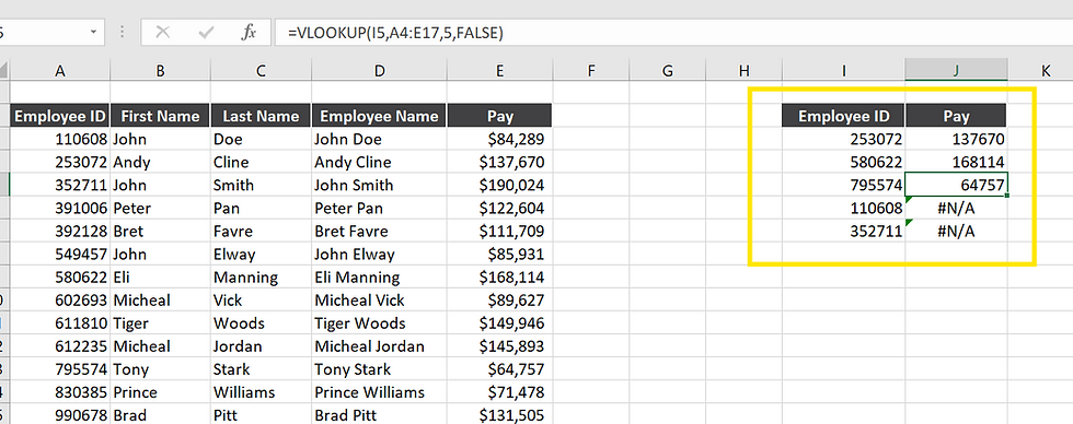
So we encounter with a problem, we got 'N/A' for some rows. When we click on to the formula we see the table has moved down two rows. And its completely missing the Employee ID's - 110608 and 352711.
So what happened is when we copied the formula by few rows the table reference also moved down by the few rows. Its called a relative reference.
In order to solve this we can lock the reference to the table by clicking on the 'Pay' for the initial formula and adding a '$' before each table reference ('F4' short cut key) as follows:

Now after clicking 'Enter' we can copy the formula to other rows by dragging it down. Now it works as expected by adding the exact values for Pay for each employee.

One problem with the above technique is if we add additional rows or remove rows this reference is no longer accurate. And we will have to come and update it every time we add or remove data.
Let's see another technique for the same :
Delete the rows for 'Pay' again in the smaller table and start over .
Click in to the table of data (i.e, the bigger table on the left ) and go to 'Insert' upon top and click the 'Table' icon.
Check the 'My table has headers'. Now we have formed a table.

Now reference this table in the VLOOKUP formula by selecting the entire table for the table array part in the formula :
= VLOOKUP ( I5 , Table 7 [#All] , 5 ,FALSE )
Table 7 is the table we created above and [#All] refers to the entire table.

Click ' Enter ' and it works.
Now if we add or delete more employee details to this list this formula will still point out to all of the correct list.

PIVOT TABLE :
A Pivot Table in Excel is a powerful tool that lets you quickly summarize, analyze the datasets without complex formulas. It uses simple drag and drop options for grouping ,filtering and calculating data into meaningful values. For example, you can see the total sales by region, average revenue per product, or customer counts by category in this case total orders for each customers.
Let's Start with an example , We have Sales data for a Product ( T-Shirt Sales) with Customer, Order ID, Product , Units sold, Date , Revenue, our cost as below:

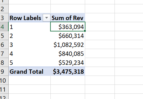
From the above table lets assume we need the Total Revenue by each customer and number of orders made by each customer ( like the already created smaller table on the right from the image above)
We can do this by applying formulas to the fields and getting the inputs or by simply using pivot table.
Start by clearing the empty rows and columns from your data if you have any and proceed.
Let's turn our current list to table. Go to Insert-> Table ( Ctrl +T)
Your table will be automatically selected and check the 'My Table has Header ' and click 'Ok'.
The table will be created within the sheet and rename it to 'Sales Data'

Now we can start creating our Pivot table
Go to Insert-> Pivot Table.
When we click on it asks what we have to include as a part of our pivot table .So we include our table 'Sales Data' and choose 'New worksheet' and click 'OK'

Now we have a new sheet with pivot table created like below:

Click on the pivot table and over on the right hand side we have a pivot table fields in a pane.
These fields will match out table columns . We have to click and drag these fields in order to build our pivot table i.e, Sales revenue and order details for each customer.
We have to recreate the smaller table we have already created using formulas.
Since we have to create Customer ID and generate Revenue for each customer. We drag on the 'Customer' field to 'Rows' and 'Revenue' to 'Values ' and change it to sum.
Here in the 'Values' pane we have multiple options for displaying our values like sum, count, average and so on.

Now we have generated the Total Revenue for each customer but the formatting seems off.
So Right-Click on the revenue and 'Number format' it to 'Currency' and change the decimal places.

Since we have to create Order ID as next field for each customer. We drag on the 'Order ID' field to 'Values' .
We have to get the count values so right-click on the orders and summarize the values to 'Count' .
We have generated our basic pivot table.


So we can do much more with pivot tables since it doesn’t just give quick summaries, it also lets you add charts, apply filters, and drill down into specifics. For example, you can move from seeing overall sales to a detailed view, such as T-shirt sales for each customer, helping you uncover patterns and insights more easily.
We can sort the Order ID column to generate which customer has contributed to the highest revenue, also add %of Revenue and so on.

We can also drag the 'Product ' to columns and change the design and colors to the table.

Conclusion :
VLOOKUP is great for pulling the right pieces of data together, while Pivot Tables make it simple by creating pivot tables for organizing and exploring that data. Used together, they turn Excel into a simple and a powerful way to compare results and answer real business questions.
Thank You!
Practice Dataset: