Data Visualization in Python: A Beginner’s Guide to Popular Charts


Data visualization is an important skill for every data analyst. Instead of looking at large tables of numbers, charts and graphs make data easier to understand. They help people quickly spot trends, patterns, and important information. Python offers useful tools like Pandas, Matplotlib, and Seaborn that make it simple to create charts and turn raw data into clear and meaningful visuals.
In this article, we'll explore the Popular charts that every beginner data analyst should know.
1. Bar Chart
2. Line Chart
3. Pie Chart
4. Histogram
5. Scatter Plot
6. Box Plot
7. Area Chart
8. Heatmap
First Let us see, When to use each type of chart:
CHART TYPE | BEST FOR |
Bar Chart | Comparing Categories |
Line Chart | Showing Trends Over Time |
Pie Chart | Displaying Proportions |
Histogram | Understanding Data Distribution |
Scatter Plot | Finding Relationship Between Variables |
Box Plot | Summarizing data distribution and detecting outliers |
Area Chart | Showing trends while emphasizing the total magnitude or cumulative values. |
Heat Map | Show patterns, relationships or intensity levels using colors |
1. Bar Chart:
When you need to compare data from different categories, a bar chart is often the best choice. It presents information using rectangular bars, helping viewers quickly understand differences and trends in the data.
Practical Examples:
Comparing product sales
Survey results
Revenue by department
Python Code for Creating Bar Chart:
import matplotlib.pyplot as plt
products = ['A', 'B', 'C', 'D']
sales = [120, 150, 90, 200]
plt.bar(products, sales)
plt.title('Product Sales')
plt.xlabel('Products')
plt.ylabel('Sales')
plt.show()
Advantage:
Bar charts make it easy to compare values and quickly identify the highest and lowest performers.
2. Line Chart:
When you want to see how something changes from one time period to another, line chart is a great choice. It connects data points with lines to clearly show trends.
Practical Examples:
Monthly sales trends
Website traffic analysis
Stock price movements
Python Code for Creating Line Chart:
import matplotlib.pyplot as plt
x = [1, 2, 3, 4, 5]
y = [50,52,51,55,53]
plt.plot(x, y, marker='o', linestyle='-', color='b', label='Sales')
plt.title('Stock Price Movement')
plt.xlabel('Days')
plt.ylabel('Stock Price')
plt.show()
Advantage:
Line charts allow analysts to see how data moves over time, making it easier to identify patterns, measure progress, and detect repeating trends.
3. Pie Chart:
Pie charts are used to display how a whole is divided among different categories. Each slice represents a category's contribution to the total.
Practical Examples:
Market share analysis
Budget allocation
Customer segmentation
Python Code For Creating Pie Chart:
import matplotlib.pyplot as plt
color = ['Red', 'Blue', 'Green', 'yellow']
respondents = [40,30,20,10]
custom_colors = ['#FF0000','#0000FF','#008000','#FFFF00']
plt.pie(respondents, labels=color,colors=custom_colors)
plt.title('Survey Respondents by Favorite Color')
plt.show()
Advantage:
Pie charts are useful for showing proportions and percentages in an easy-to-understand format.
4. Histogram:
A histogram displays the pattern of numerical data, making it easier to see where most values are concentrated and how the data is distributed.
Practical Examples:
Employee salaries
Exam scores
Customer age distribution
Python Code For Creating Histogram:
import matplotlib.pyplot as plt
scores = [55, 60, 65, 70, 72, 75, 80, 82, 85, 90, 95]
plt.hist(scores, bins=5)
plt.title('Exam Score Distribution')
plt.xlabel('Scores')
plt.ylabel('Frequency')
plt.show()
Advantage:
Histograms make it easier to see how data is distributed, where most values are grouped, and whether there are any unusual values.
5. Scatter plot:
Scatter plots are used to examine how one variable changes in relation to another. They help reveal whether a relationship exists between the two variables.
Practical Examples:
Advertising spend vs. sales
Study hours vs. exam scores
Temperature vs. electricity usage
Python Code For Creating Scatter Plot:
import matplotlib.pyplot as plt
study_hours = [1, 2, 3, 4, 5, 6, 7]
scores = [50, 55, 60, 70, 75, 85, 90]
plt.scatter(study_hours, scores)
plt.title('Study Hours vs Exam Scores')
plt.xlabel('Study Hours')
plt.ylabel('Exam Scores')
plt.show()
Advantage:
Scatter plots reveal how two sets of data interact, making it easier to spot trends, connections, and relationships.
6. Box Plot:
A Box Plot is a chart that gives a quick overview of a dataset. It shows the smallest value, largest value, middle value (median), and how the data is spread across different ranges. Also Called as Whisker Plot. This makes it easy to understand the distribution of data and identify any unusual values.
Practical Examples:
Employee Salaries by Department
Product Delivery times
Stock Returns
Python Code For Creating Box Plot:
import pandas as pd
import matplotlib.pyplot as plt
data = { "CustomerID": [1, 2, 3, 4, 5, 6, 7, 8, 9, 10, 11], "City": ["NY", "NY", "NY", "LA", "LA", "LA", "CH", "CH", "CH", "CH", "CH"] }
df = pd.DataFrame(data)
df.boxplot(column="CustomerID", by="City”)
plt.title("Customer’s City")
plt.ylabel("Age")
plt.show()
Advantage:
Box Plot summarizes large amounts of data and highlights outliers, making it easy to compare distributions across different groups.
7. Area Chart:
An area chart is very similar to a line chart, but the space between the line and the horizontal (x) axis is filled with color or shading. This makes it easier to see not only the trend over time but also the magnitude of the values being represented.
Practical Examples:
Tracking sales growth over time
Monitoring website traffic
Showing revenue trends
Python Code For Creating Area Chart:
import pandas as pd
import matplotlib.pyplot as plt
data = { 'Sales': [10, 15, 23, 18, 25], 'Marketing': [5, 8, 12, 14, 19] }
df = pd.DataFrame(data, index=[2021, 2022, 2023, 2024, 2025])
df.plot.area(alpha=0.4)
plt.title("Company Expenses Over Time")
plt.ylabel("Amount in $")
plt.show()
Advantage:
Area Chart shows trends over time while also emphasizing the total amount or volume of the data.
8. Heat Map:
A heatmap is a graphical representation of data where individual values are represented by color intensity.
Practical Examples:
Student Performance Analysis
Website Traffic Analysis
Correlation Matrix
Python Code for Creating Heat Map:
import numpy as np
import matplotlib.pyplot as plt
data = np.random.rand(5, 5)
fig, ax = plt.subplots()
cax = ax.imshow(data, cmap='plasma')
fig.colorbar(cax)
plt.show()
Advantage:
Heat Map uses colors to make patterns, trends, and relationships in large datasets easy to spot at a glance.
Things To Remember For Better Output:
Few codes to keep in mind while creating charts, no matter what type of chart we create keeping this following three lines of code makes our chart readable:
plt.title(): Tell the audience exactly what they are looking at.
plt.xlabel() and plt.ylabel(): Label your axes so the numbers actually mean something.
plt.show(): Cleanly render and display your image.
To Conclude, Learning these popular basic charts is an excellent starting point for any aspiring data analyst. These charts can help you answer a wide range of business and analytical questions. By mastering these visualizations in Python, you'll be able to turn raw data into meaningful insights and communicate your findings more effectively.