A beginner’s hands-on comparison of join, relationship, blend and union

By Poulami Chakraborty
When I started learning Tableau, "join", "relationship", "blend" and "union" all sounded like different names for the same thing. Reading definitions only took me so far, so I learned them the way I learn most things: by trying each one on data where I already know the right answer. Tableau will give you a number whichever method you pick, so the real skill is checking whether that number is correct.
So I built a tiny dataset and tried all four methods on it, one step at a time. This post walks through exactly what I clicked, what I saw, and what the numbers told me. If you are at the same stage I am, this should save you a few confused evenings.
• Relationship: the default. Start here whenever both tables are in the same source.
• Join: use it when you need one flat table, and check your totals afterwards.
• Blend: use it only when the data is in different sources.
• Union: use it to stack rows from tables that have the same columns.

The sample data
I made three small tables across two Excel files:
• Orders (in Sample.xlsx): 25 orders with OrderID, Region and Sales, across four regions: East, West, North and South.
• Returns (in Sample.xlsx): 20 return rows with OrderID, Reason and Refund. Four orders (1001, 1005, 1008 and 1016) were returned twice, which is on purpose. It is the trap that makes joins misbehave.
• Targets (in Targets.xlsx): one sales target per region.
The true sales per region, calculated from the Orders table alone, are:
Region | True Sales |
East | 1,075 |
North | 1,020 |
South | 1,120 |
West | 1,185 |
Keep these numbers in mind. They are the answer key for everything below.
The four methods in one minute
• Join: Tableau physically merges two tables into one wide table, row by row, before anything is summed.
• Relationship: the tables stay separate. Tableau links them on a field and works out the join for each chart, summing each table at its own level first.
• Blend: the tables come from different data sources. Tableau summarizes each source on its own, then lines the results up on a shared field.
• Union: the opposite direction. Tableau stacks tables that have the same columns on top of each other, so you get more rows instead of more columns.
What is a physical table?
A physical table is a real table that already exists in your data source: a sheet in an Excel workbook, a CSV file, or a table in a database. In my files, Orders and Returns are each one physical table. Tableau reads them exactly as they are stored.
Tableau has two layers on the Data Source tab. The physical layer is where physical tables are merged into a single flat table using joins (or stacked using unions). You get there by double-clicking a table on the canvas. The logical layer is the top-level canvas, where each box is a logical table. A logical table can be made of one physical table or of several physical tables that were joined together, and relationships connect logical tables to each other.
Here is how that plays out in this post. When I join Orders and Returns in Part 1, the two physical tables get merged into one logical table, and Tableau labels it "Orders is made of 2 tables". When I use a relationship in Part 2, Orders and Returns stay as two separate logical tables, each backed by one physical table.
Join
Step 1: Connect and open the physical layer
I connected to Sample.xlsx, then double-clicked the Orders box on the canvas. That takes you into the physical layer, which is where joins live. The box now says that Orders is made of 1 table.

Step 2: Drag Returns next to Orders
I dragged Returns from the Sheets list on the left onto the canvas. A join icon appeared between the two tables, two overlapping circles. The text changes to "Orders is made of 2 tables". Tableau picks an Inner join by default, which is why only the overlapping part of the circles is filled in.

Step 3: Open the join and check the key
I clicked the join icon to open the Join panel. The join clause reads Order ID on the Orders side, equals, OrderID (Returns) on the Returns side. Tableau had tidied the field name in Orders to "Order ID", but it is the same OrderID column.

Step 4: Switch from Inner to Left
An Inner join keeps only the orders that have a matching return, so I would silently lose every order that was never returned. I clicked Left instead, which keeps all 25 orders and attaches returns where they exist. The Venn picture changes so that the left circle is filled in.

Step 5: Build the view, and spot the problem
I clicked Sheet 1, dragged Region to Rows and Sales to Text. The totals came out as:
Region | Join result | True value |
East | 1,175 | 1,075 |
North | 1,540 | 1,020 |
South | 1,300 | 1,120 |
West | 1,185 | 1,185 |
Only West is right. Here is what happened. Orders 1001, 1005, 1008 and 1016 each have two return rows, so the join copies each of those orders onto two rows. The 25 orders turned into 29 rows, and each copy carried the full sales amount. For example, order 1001 is worth 100, but it now shows up
twice in East, which adds 100 too much (1,075 plus 100 gives 1,175). West was safe only because none of its orders had two returns.

Tableau did not show an error. The numbers just looked normal.
Step 6: Fix it with a calculated field
I created a calculated field called Sales Fixed (Analysis menu, then Create Calculated Field):
[Sales] / {FIXED [Order ID] : COUNT([Order ID])}
The idea is simple. For order 1001, the COUNT is 2 because it appears on two rows, so each row now holds 100 / 2 = 50. When Tableau adds the two rows back together, you get 100 again. Orders that appear on a single row are divided by 1, so nothing changes for them.

Step 7: Check the corrected totals
I replaced SUM(Sales) with SUM(Sales Fixed) in the view. The numbers now match the answer key: East 1,075, North 1,020, South 1,120 and West 1,185. Tableau shows them with a dollar sign because the new field picked up currency formatting, which is cosmetic.

Lesson: a join works, but when one side has several rows per key, you have to protect your sums yourself.
Relationship
Step 1: Start in the logical layer
I opened a fresh data source on Sample.xlsx and double-clicked Orders onto the canvas, but this time I did not double-click into it. This top-level canvas is the logical layer, and it is where relationships are made. The data grid below shows 3 fields and 25 rows, which matches my Orders table.

Step 2: Drag Returns beside Orders
I dragged Returns next to Orders. Instead of a join icon, Tableau draws a plain line between the two boxes. That line is the relationship, sometimes called the noodle.

Step 3: Check the linking field
I clicked the line. At the bottom, Tableau shows Order ID in Orders, an equals operator, and OrderID (Returns) in Returns. I left the Performance Options at their defaults. Below the grid I can also see all the Returns rows, including the two return rows for orders like 1001 and 1005. There is a red Remove Relationship button if you ever need to undo it.

Step 4: Build the view
I went to Sheet 1, dragged Region to Rows, then Sales and Refund to Text. The result:
Region | Sales | Refund |
East | 1,075 | 120 |
North | 1,020 | 180 |
South | 1,120 | 175 |
West | 1,185 | 205 |
The sales match the answer key, with no calculated field needed. In the Data pane, Orders and Returns also appear as two separate tables, each with its own count, instead of one merged table.

Why it works: Tableau sums Sales from Orders on its own and Refund from Returns on its own, and only then lines them up by region. The duplicate return rows never get a chance to multiply the sales.
Blend
For the blend, Targets lives in a completely different file, so Orders and Targets are two separate data sources.
Step 1: Build a view from the first source
I connected to Sample.xlsx with just the Orders table, then built Region in Rows and SUM(Sales) in the view. The Data pane shows the source name, Orders (Sample), at the top. Once I used a field from this source in the sheet, Tableau marked it with a blue check mark.

Step 2: Add a new data source
I opened the Data menu and chose New Data Source (shortcut Ctrl+D). Notice the menu also has "Edit Blend Relationships", which is greyed out until a second source exists.

Step 3: Connect to the Targets file
On the Connect screen, under To a File, I clicked Microsoft Excel and picked Targets.xlsx.

Step 4: See both sources in the Data pane
Back on Sheet 1, the Data pane now lists two sources: Orders (Sample) and Targets (Targets). I clicked Targets to select it. Next to its Region field there is a small chain icon. That icon is the link that tells Tableau how to line the two sources up. Both sources have a field called Region, so Tableau uses it as the link.

Step 5: Drag Target into the view
With Targets still selected, I dragged Target onto the sheet. It appears as SUM(Target) under each region's sales: East 900, North 1,000, South 1,100 and West 1,200. The moment I used a field from Targets, that source picked up an orange check mark.

Step 6: Look at the final picture
In the final screenshot you can see the whole story: Orders (Sample) with the blue check, Targets (Targets) with the orange check, and a small orange mark on the SUM(Target) pill itself.

What do the blue and orange checks mean?
This was the part that confused me the most, so here it is plainly:
• Blue check = primary data source. It is the source whose field you used first on this worksheet. It decides which rows show up. In my example, Region comes from Orders, so the sheet lists the regions that exist in Orders.
• Orange check = secondary data source. It is any other source you pull a field from after that. Its numbers are looked up and attached to whatever the primary source already shows. Pills that come from the secondary source also carry a small orange mark, like SUM(Target) did.
• The chain icon next to a field is the link between the two sources. A grey, broken-looking chain means the link exists but is not switched on. A red or orange chain means the link is active, and clicking the chain toggles it. In my case Tableau had already matched Region on its own, so my targets lined up straight away. If yours shows a broken chain and the targets show as blank or an asterisk, click it.
A few things that are good to know:
1. Order matters. If I had dragged a Targets field into the sheet first, Targets would have become primary and Orders secondary. With only four regions in both, I would not have seen a difference here, but with real data, the primary source controls which rows appear.
2. It is per worksheet. A source can be primary on one sheet and secondary on another.
3. The secondary source is always summarized first. That is why a blend cannot do row-level things that a join or a relationship can.
Union
A union is the odd one out. A join, a relationship and a blend all line up rows from different tables and bring in more columns. A union does the opposite: it stacks tables that have the same columns on top of each other, so you end up with more rows. Think of monthly sales files, or the same report exported in batches, that you want in one table.
For this I made a file called Orders_Union.xlsx. It holds the same 25 orders as before, split across two sheets with identical columns (OrderID, Region and Sales): Orders_Batch1 has 13 rows (orders 1001 to 1013) and Orders_Batch2 has 12 rows (orders 1014 to 1025).
Step 1: Connect to the file
I clicked Microsoft Excel under Connect and selected Orders_Union.xlsx. The Data Source tab lists Orders_Batch1 and Orders_Batch2 under Sheets on the left.
Step 2: Open the Union dialog
I double-clicked New Union, just below the sheet list. The dialog has two tabs, Specific (manual) and Wildcard (automatic). I stayed on Specific.

Step 3: Add both sheets
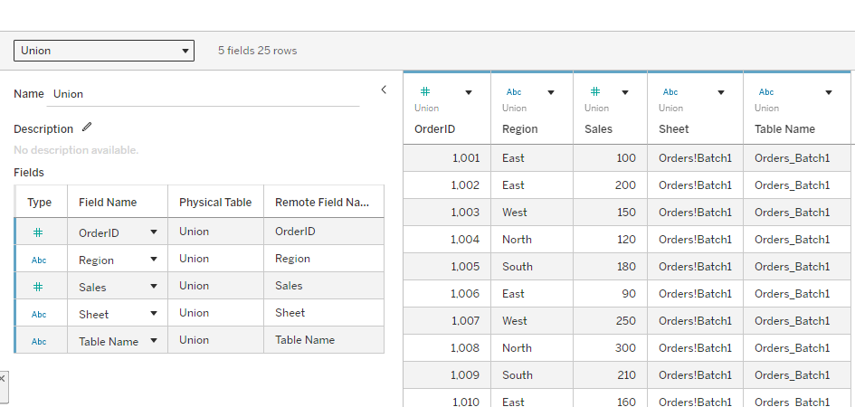
I dragged Orders_Batch1 into the dialog, then Orders_Batch2 under it, and clicked Apply, then OK. Tableau stacks them into one logical table, built from two physical tables.

Step 4: Check the stacked rows
The grid under the canvas shows 25 rows, which is 13 plus 12. Next to OrderID, Region and Sales, Tableau adds two helper fields, Sheet and Table Name. They record where each row came from. In the Table Name column, orders 1001 to 1013 show Orders_Batch1 and the rest show Orders_Batch2.
Step 5: Build the view and check the totals
On Sheet 1, I dragged Region to Rows and Sales to Text. The totals match the answer key exactly: East 1,075, North 1,020, South 1,120 and West 1,185. Nothing was duplicated, because a union only adds rows and never matches them.

Step 6: Split the totals by source sheet
I dragged Sheet to Columns, which splits each region into the two batches it came from:
Region | Orders_Batch1 | Orders_Batch2 | Total |
East | 550 | 525 | 1,075 |
North | 515 | 505 | 1,020 |
South | 665 | 455 | 1,120 |
West | 530 | 655 | 1,185 |
One thing to watch out for
A union lines columns up by name. If a column is spelled differently in one sheet, for example Sales in one and Sale in another, Tableau puts it in its own column and fills the other sheet's rows with nulls. Keep your headers identical.
Lesson: use a union when the tables have the same columns and you need more rows. Use a join, relationship or blend when you need more columns.
Bonus: See the merged data and swap data sources
Two questions came up while I was testing. Can I actually see the merged dataset, and can I flip the same chart from one method to another without rebuilding it? Yes to both. One warning first: Replace Data Source does not merge anything. It swaps the data source behind a worksheet, and the merging is still done by the join, the relationship or the blend.
See the merged dataset
1. Join: on the Data Source tab, the grid under the canvas shows 6 fields and 29 rows. Order 1001 appears on two rows, one for Damaged (20) and one for Late (30). This is the duplication from Part 1, now visible.
2. From a sheet: open the Data menu, choose the data source name, then View Data, and open the Full Data tab to see every row.
3. Relationship: click the Orders box, then the Returns box. The grid shows one table at a time, 25 rows for Orders and 20 for Returns. There is no single merged table, which is why the sums stay correct.

Swap the data source with Replace Data Source
1. Choose Data, then New Data Source, then Microsoft Excel, and select Sample.xlsx again. Drag Orders onto the canvas, then Returns beside it to make a relationship.
2. Right-click each data source in the Data pane, choose Rename, and call them Join version and Relationship version. Two sources with the same name are easy to mix up.
3. On Sheet 1, select Join version in the Data pane. Put Region on Rows and SUM(Sales) on Text.
4. With Join version still selected, open Data, then Replace Data Source. Set Current to Join version and Replacement to Relationship version, then confirm.
5. Tableau matches fields by name, so Region and Sales carry over and the same chart redraws on the new source.
Any pill that exists only in the old source, such as Sales Fixed, turns red with an exclamation mark. Remove it. To flip back, run the same steps in reverse.


What changes
The chart, the pills and the layout stay the same. Only the data source behind them changes:
Region | Join version | Relationship version |
East | 1,175 | 1,075 |
North | 1,540 | 1,020 |
South | 1,300 | 1,120 |
West | 1,185 | 1,185 |
I like this exercise because it shows the problem without any calculation. The same SUM(Sales) pill gives two different answers, and the only thing I changed was how the tables were combined.
Putting it all together
| Join | Relationship | Blend | Union |
Where it happens | Physical layer | Logical layer | Worksheet | Physical layer |
Data sources | Same | Same | Different | Same |
Combines | Row by row, before summing | At query time, per chart | After summing | Stacks rows of tables with the same columns |
Risk | Duplicate rows inflate totals | Few | Limited features, primary decides rows | Mismatched column names create null-filled columns |
East sales in my test | 1,175 (wrong) | 1,075 | 1,075 with target 900 | 1,075 (550 + 525) |
My rule of thumb after this experiment:
1. If both tables are in the same source, start with a relationship.
2. Use a join when you really need one flat table, and always check your totals against the original table afterwards.
3. Use a blend only when the data is in different sources and cannot be combined any other way.
4. Use a union when the tables have the same columns and you simply need more rows, such as one sheet per month.
The one habit to take away
Whenever you combine tables, compare one total in Tableau against the original table. I only caught the join problem because I knew East's true sales were 1,075. If I had not checked, I would have trusted 1,175 and never known.