WINDOW FUNCTIONS : The Analyst’s Secret Weapon

Feb 12

7 min read

WHY ANALYSTS NEED WINDOW FUNCTIONS?

Before we deep dive into what a window function is, the syntax and how to write it, let us understand why we even need a window function.

When you work for a company, as an analyst, you’re constantly asked things like:

“How does this row compare to others?”
“What has changed since last week?”
“What’s the running total?”
“Who’s top-N within each group?”
“What’s this user’s previous / next event?”

A classic SQL (GROUP BY) can’t answer those cleanly, because it collapses rows. But the Window functions let you add context to each row without losing detail. So, Analysts need window functions because they:

Preserve row-level detail
Add powerful comparisons
Replace big and complex subqueries
Make SQL expressive instead of painful

What is a Window Function?

A window function performs a calculation across a set of table rows that are somehow related to the current row. This is comparable to the type of calculation that can be done with an aggregate function. But unlike regular aggregate functions, use of a window function does not cause rows to become grouped into a single output row — the rows retain their separate identities. Behind the scenes, the window function is able to access more than just the current row of the query result.

GROUP BY vs WINDOW FUNCTION

GROUP BY

The GROUP BY clause is used with aggregate functions (like AVG, SUM, COUNT) to group the result set by one or more columns.

WINDOW FUNCTIONS

Window functions perform a calculation across a set of table rows that are related to the current row. Unlike GROUP BY, all original rows are preserved in the output.

Feature	GROUP BY	Window Functions
Row Count Usage	Reduces the number of rows (1 per group). Creating high-level summary reports.	Retains all original rows. Comparing individual rows to group aggregates.
Attributes	Can only select columns in GROUP BY aggregates.	Can select any column or alongside the calculation.
Analogy	A "Summary" or "Total" row.	Adding a "Running Total" or "Rank" column to a list.

Lets see this with examples,

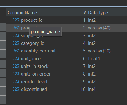
We have taken a product table of a store dataset to execute our queries.

GROUP BY:

Result:

The output has only one row per category. You cannot see individual products here because they are "collapsed" into the average.

While using a window function,

Result:

Example 2: Using RANK()

The unit_price of each product is ranked category wise.

Understanding the basic Syntax of Window Functions:

Basic Syntax:

SELECT <column_1>, <column_2>,

<window_function(expression)>

OVER ( PARTITION BY <...>

ORDER BY <...>

<window_frame>)

<window_column_alias>

FROM <table_name>;

Note: Not every part is required, but this is the full shape.

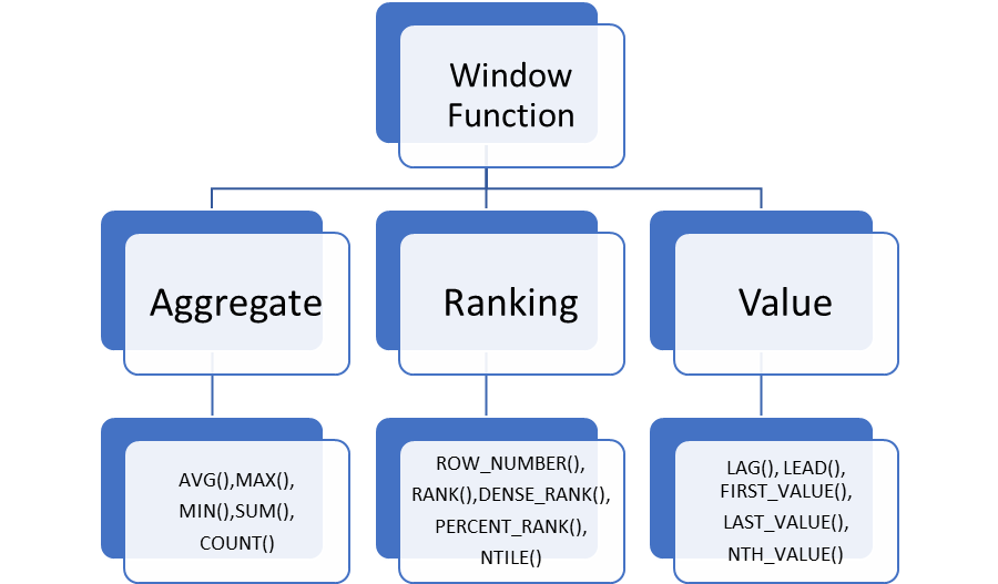
Components:

window_function(expression) → SUM, AVG, ROW_NUMBER, etc.
OVER(..) → the Magic part
PARTITION BY → groups rows logically
ORDER BY → defines sequence
window_frame → fine-tune the window (advanced but powerful)
window_column_alias → name of the new resulting column.

Components in detail:

window_function (expression):

This is the function you want to apply across a set of rows, instead of collapsing them like GROUP BY.

Common window functions are, Aggregate-style functions like SUM(), AVG(),MIN(), MAX(), etc., Ranking functions and Value access functions like LAG(), LEAD(), etc.,

OVER (...) - The Magic Part:

OVER tells SQL: “Do this calculation over a window of rows, but keep every row in the result.” Without OVER, it’s just a normal aggregate.

PARTITION BY - split the data

This divides rows into independent groups, kind of like GROUP BY, but without collapsing rows.

Example:

AVG(unit_price) OVER (PARTITION BY category_id)

Calculates average of unit prices per category, but still shows every product.

If you omit PARTITION BY, the function runs over the entire table.

ORDER BY — define row order inside the window

This is required for ranking and running totals.

Example: (ORDER BY hire_date)

ROW_NUMBER() OVER (ORDER BY hire_date)

Numbers rows based on hire date.

With aggregates:

SUM(salary) OVER (ORDER BY hire_date)

Running total of salary.

frame_clause — fine-tune the window (advanced concept but powerful)

This controls which rows around the current row are included for the calculation. We will see this in detail later.

Lets see some more examples for better understanding,

NTILE() Function:

The NTILE(n) function divides an ordered partition into n buckets (groups) and assigns a bucket number to each row. This is commonly used for creating quartiles or percentiles.

Scenario: You want to group all products into 4 price quartiles (from most expensive to cheapest).

Result:

What this does:

It sorts all products by price.
It splits the total list into 4 equal groups.
The top 25% of expensive products get assigned 1, the next 25% get 2, and so on.

LAG() Function:

The LAG() is excellent for comparing a value in the current row with a value in a previous row.

Scenario: Within each category, you want to see a product's price and the price of the "next most expensive" product to see the price gap.

Result:

What this does:

PARTITION BY category_id: Resets the calculation for every category.
ORDER BY unit_price DESC: Sorts products from high to low.
LAG(unit_price ): Looks at the row immediately above the current one.

Lets get back to the syntax. So far in our examples we never used this window_frame clause.

What a frame clause actually does?

The frame clause is used with window functions to define the subset of rows within the partition that the function operates on. It controls the “window” or range of rows that are considered for the calculation of each row’s result.

Inside a window function, you have two levels of “scope”:

Partition is, Which rows belong to my group?
Frame is, Which rows from that group are used for this row’s calculation?

For each row, the frame clause defines a sliding window of rows around it.

Syntax:

OVER ( PARTITION BY ...

ORDER BY ...

frame_type BETWEEN frame_start AND frame_end

)

Where:

frame_type = ROWS | RANGE | GROUPS
frame_start / frame_end define the boundaries

This is one of the most misunderstood but most powerful parts of window functions.

The frame clause answers the question: "For the current row, exactly which rows are included in the calculation?"

The three keywords — ROWS, RANGE, and GROUPS — define how that frame is built.

They differ in what “neighboring rows” means.

Understanding will be better with the following examples.

Example using the keyword ROW to define the frame.

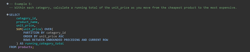
Goal: Within each category, calculate a running total of the unitPrice as you move from the cheapest product to the most expensive.

Result:

As breaking down the Frame Clause:

PARTITION BY category_id: Groups the calculation by category.
ORDER BY unit_price ASC: Sets the direction of the "flow" for the running total.
ROWS BETWEEN UNBOUNDED PRECEDING AND CURRENT ROW: This is the frame. It tells PostgreSQL, "For every row, sum the price of everything from the very start of this category up to the row I am standing on right now."

Like the above explained frame clause, we can also find moving average, remaining balance etc.,

ROWS BETWEEN 1 PRECEDING AND 1 FOLLOWING: A 3-row "moving average" or window (looks at the previous row, current row, and next row).
ROWS BETWEEN CURRENT ROW AND UNBOUNDED FOLLOWING: Looks from the current row to the end of the group (useful for "remaining balance" style calculations).
ROWS 3 PRECEDING: Short form of ROWS BETWEEN 3 PRECEDING AND CURRENT ROW

RANGE:

The RANGE clause defines the window frame based on logical values rather than a fixed number of physical rows (which is what ROWS does). If multiple rows have the same value in the ORDER BY column, RANGE treats them as a single group (peers). This is particularly useful when dealing with prices or dates where ties occur.

Example using the keyword RANGE to define the frame.

RANGE:

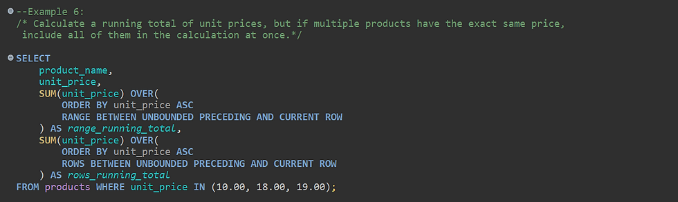
Goal: Calculate a running total of unit prices, but if multiple products have the exact same price, include all of them in the calculation at once.

Result:

As breaking down the Frame Clause:

ROWS (Physical): Adds the price row-by-row. In the second row, the total is just $18 + $18 = $36.
RANGE (Logical): Sees that four rows share the "Current Row" value of $18.00. It treats them as a single peer group and adds all of them to the total immediately. All items with the same price get the same running total ($72.00).

Default Behavior: In PostgreSQL, if you use ORDER BY in a window function but omit the frame clause, the default is RANGE BETWEEN UNBOUNDED PRECEDING AND CURRENT ROW. If you want a row-by-row cumulative sum regardless of duplicate values, you must explicitly use ROW

Example using the keyword GROUP to define the frame.

Goal: For each product, calculate the average price of its own price group and the group of products immediately preceding it in price.

Result:

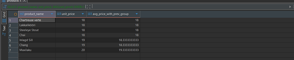
How GROUPS Works here:

The First Group ($18.00): There are 4 products priced at 18.00. Since there is no "1 preceding" group, the average is just (18+18+18+18) / 4 = 18.00.
The Second Group ($19.00): There are 2 products priced at 19.00 (Chang and Gula Malacca). The frame includes this group PLUS the "1 preceding" group ($18.00). The average is calculated across all 6 products in these two groups.
The Third Group ($20.00): The frame includes the $20.00 group and the "1 preceding" group ($19.00). It effectively "slides" by sets of identical values.

Named Window Function:

Is nothing but defining the window once, reuse it many times.

Syntax:

SELECT <column_1>, <column_2>,

<window_function>() OVER <window_name>FROM <table_name>

WHERE <...>

GROUP BY <...>

HAVING <...>

WINDOW <window_name> AS (

PARTITION BY <...>ORDER BY <...> <window_frame>)

ORDER BY <...>;

Example:

SELECT country, city,

rank() OVER country_sold_avg FROM sales

WHERE month BETWEEN 1 AND 6

GROUP BY country, city

HAVING sum(sold) > 10000

WINDOW country_sold_avg AS (

PARTITION BY country

ORDER BY avg(sold) DESC)

ORDER BY country, city;

Example with our products table,

Result:

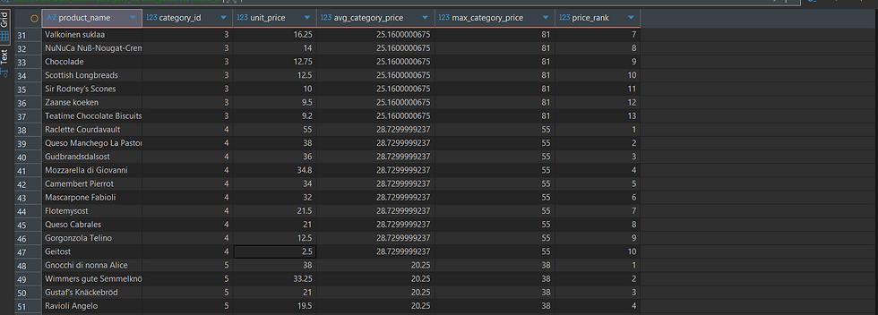
Final Takeaway:

✨Window functions elevate SQL from a querying language to a true analytics engine. They enable advanced calculations—ranking, running totals, comparisons, and trend analysis—without complex joins or subqueries.

✨ They preserve the original dataset. Unlike GROUP BY, window functions perform powerful calculations without collapsing rows, keeping every detail intact while adding analytical depth.

✨ hey’re a must-have skill for every analyst. Mastering window functions unlocks cleaner queries, smarter insights, and more efficient problem-solving.

Conclusion:

When you can analyze trends, rank performance, compare across partitions, and calculate rolling metrics—all without losing granular data—that’s not just SQL anymore.

That’s why window functions truly are the analyst’s secret weapon.

"Window functions are the difference between

knowing SQL and thinking like an analyst.”