Unlocking the Power of Power BI: Essential Functions for Data Analysis


In the world of data analysis and visualization, Power BI shines as a robust tool that helps users uncover meaningful insights from their data. A key feature that enhances Power BI’s functionality is DAX, or Data Analysis Expressions. DAX is a specialized formula language that allows users to build custom calculations, making it possible to create calculated columns, measures, and tables within their data models.
Difference Between Power Query and DAX
Power BI relies on two key languages for data manipulation: Power Query and DAX.
Power Query: Focuses on data transformation and shaping, allowing users to connect to various data sources, clean, transform, and load the data into Power BI.
DAX: Handles calculations and analysis within the data model, enabling users to perform dynamic and advanced computations.
Both languages are essential for creating effective data models in Power BI. Power Query prepares the data, while DAX performs calculations and analysis on the transformed data.
Dataset Overview
To demonstrate DAX functions, we use the following tables:
Sales Table
Products Table
Sales Table

Products Table

Functions
1. RELATED
The RELATED function fetches values from a related table, enabling seamless integration between connected datasets.
Syntax:
RELATED(<column>)
Steps:
Ensure a relationship exists between the relevant tables.
Create a new column in the target table.
Use RELATED to fetch the desired column value.
Example: Adding Product Name to Sales Table
Product Name = RELATED(Products[Product Name])
Output:
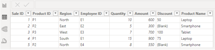
Explanation: RELATED leverages the established relationship to bring data from the Products table into the Sales table.
2. SUM
The SUM function adds all numbers in a specified column.
Syntax:
SUM(<column>)
Steps:
Create a new measure in the Sales table.
Use SUM to calculate the total value of a numeric column.
Example: Total Sales
Total Sales = SUM(Sales[Amount])
Output:
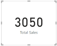
Explanation: SUM is a simple aggregation function that totals all values in the specified column.
3. SUMX
The SUMX function iterates over a table, evaluating an expression for each row, and then sums the results.
Syntax:
SUMX(<table>, <expression>)
Steps:
Create a new measure in the Sales table.
Use SUMX to perform row-by-row calculations and aggregation.
Example: Total Revenue
Total Revenue = SUMX(Sales, Sales[Quantity] * RELATED(Products[Unit Price]))
Output:

Explanation: SUMX calculates revenue (Quantity × Unit Price) for each row and then sums the results, making it ideal for row-level calculations.
4. CALCULATE
The CALCULATE function modifies the filter context of an expression.
Syntax:
CALCULATE(<expression>[, <filter1>][, <filter2>]...)
Steps:
Create a new measure in the Sales table.
Use CALCULATE to apply filters to an expression.
Example: Total Sales in the North Region
Total Sales North = CALCULATE(SUM(Sales[Amount]), Sales[Region] = "North")
Output:
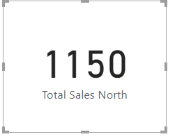
Explanation: CALCULATE evaluates the sum of the sales amount only for rows where the region is "North".
5. IF & SWITCH
IF: Evaluates a condition and returns values based on the result.
SWITCH: Returns results based on multiple conditions.
Syntax (IF):
IF(<logical_test>, <value_if_true>[, <value_if_false>])
Syntax (SWITCH):
SWITCH(<expression>, <value1>, <result1>, ..., <else>)
Steps:
Use IF for binary conditions and SWITCH for multiple conditions.
Create a calculated column to store the result.
Example (IF): Flagging High Sales
High Sales Flag = IF(Sales[Amount] > 500, "High", "Low")
Output:
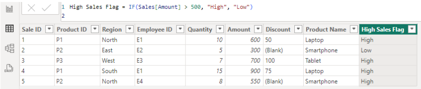
Explanation: The IF function evaluates whether the Amount column in the Sales table is greater than 500. If true, it returns "High"; otherwise, it returns "Low".
Example(SWITCH): Categorizing Regions
Region Category = SWITCH(
Sales[Region],
"North", "Domestic",
"South", "Domestic",
"East", "International",
"West", "International",
"Unknown")
Output:
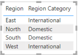
Explanation: The SWITCH function evaluates the value in the Region column. If it matches "North" or "South", it returns "Domestic". For "East" or "West", it returns "International". If no match is found, it defaults to "Unknown". Unlike IF, SWITCH is more efficient and easier to read when dealing with multiple conditions.
6. RANKX
The RANKX function ranks items in a table based on a specific expression, enabling comparison and prioritization of values.
Syntax:
RANKX(<table>, <expression>[, <value>[, <order>[, <ties>]]])
Steps:
Decide which table to rank.
Determine the metric to use for ranking.
Specify the order (ascending or descending). Default is ascending.
Handle ties with an optional parameter (SKIP, DENSE, etc.).
Example: Ranking Products by Total Sales
Product Rank = RANKX(
ALLSELECTED(Sales[Product Name]),
CALCULATE(SUM(Sales[Amount])) )
Output:
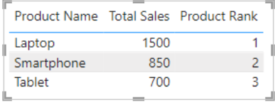
Explanation: RANKX assigns a rank to each product by evaluating the total sales. This function is useful for identifying top-performing items or entities.
7. DIVIDE
The DIVIDE function performs division and handles division-by-zero errors by returning an alternate result.
Syntax:
DIVIDE(<numerator>, <denominator>[, <alternate_result>])
Steps:
Create a new measure for calculations involving division.
Use DIVIDE to avoid errors and provide alternate results.
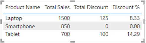
Example 1: Calculate Discount Percentage
Discount Percentage = DIVIDE(SUM(Sales[Discount]), SUM(Sales[Amount]), 0) * 100
Output1:
Example 2: Sales-to-Discount Ratio
Sales-to-Discount Ratio = DIVIDE(SUM(Sales[Amount]), SUM(Sales[Discount]), 0)
Output2:
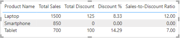
Explanation: If the denominator is zero, DIVIDE returns the specified alternate result (e.g., 0). This ensures robust calculations, even with missing or undefined data.
8. FILTER
The FILTER function returns a subset of a table based on specified criteria.
Syntax:
FILTER(<table>, <expression>)
Steps:
Use FILTER inside a calculation or with aggregation functions.
Combine it with functions like SUMX for advanced filtering.
Example: Sales Above $600
Sales Over 600 Total = SUMX(FILTER(Sales, Sales[Amount] > 600), Sales[Amount])
Output:

Explanation:
FILTER(Sales, Sales[Amount] > 600) filters rows where the Amount is greater than 600.
SUMX iterates over the filtered table to compute the total.
9. TOPN
The TOPN function returns a given number of top rows according to a specified expression.
Syntax:
TOPN(<n_value>, <table>, <expression>[, <order>])
Steps:
Create a new table or measure to extract the top N rows.
Use the TOPN function with a specific column and sorting order.
Example: Top 3 Sales
Top 3 Sales = TOPN(3, Sales, Sales[Amount], DESC)
Output:

Explanation: TOPN filters the data to retain only the top rows based on the given criteria. It is ideal for identifying best-performing entities.
10. BLANK
The BLANK function returns a blank value, commonly used in logical expressions or calculations.
Syntax:
BLANK()
Example: Replace Zero Discounts with Blank
Discount2 = IF(Sales[Discount] = 0, BLANK(), Sales[Discount])
Output:
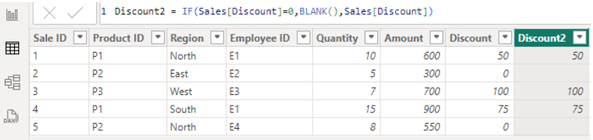
Explanation:
BLANK() creates a blank value in DAX.
Here in this example it is creating a new column where if Discount is 0 it is replaced by Blank.
It's commonly used in calculations and logical expressions to handle cases where data might be missing, or a result is undefined.
11. ISBLANK
The ISBLANK function checks whether a value is blank, returning TRUE or FALSE.
Syntax:
ISBLANK(<value>)
Steps:
Use ISBLANK to identify missing values.
Combine with IF for custom logic.
Example: Check for Missing Discounts
Discount Check = IF(ISBLANK(Sales[Discount2]), "No Discount", "Discount Applied")
Output:
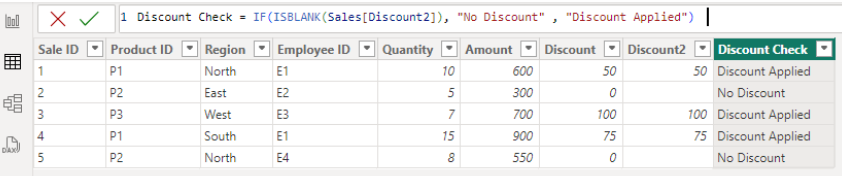
Explanation:
This formula checks if the discount2 is blank and returns a corresponding message.
Handle missing data or null values in custom measures and columns.
12. MAXX
The MAXX function calculates the maximum value of an expression evaluated for each row in a table.
Syntax:
MAXX(<table>, <expression>)
Steps:
Use MAXX to compute the maximum value based on row-level calculations.
Apply it to analyze individual rows of a table.
Example 1: Maximum Revenue Per Product
Max Revenue = MAXX(Sales, Sales[Quantity] * RELATED(Products[Unit Price]))
Example 2: Maximum Discount
Max Discount = MAX(Sales[Discount])
Output:
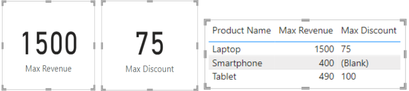
Explanation: MAXX evaluates an expression (e.g., Quantity × Unit Price) for each row and returns the highest result. MAX is a simpler version used directly on a column.
Conclusion
Mastering DAX functions in Power BI unlocks the full potential of dynamic data analysis and modeling. These functions, from basic aggregations to advanced calculations, empower users to manipulate data, handle conditional logic, and create insightful visualizations. By understanding their syntax, examples, and outputs, we can confidently build smarter, more flexible dashboards.
Whether we are filtering data, ranking values, or managing blanks, these functions offer the precision and flexibility needed to tackle complex challenges. With continued exploration and application, we can streamline our reporting process, uncover deeper insights, and drive informed decision-making with impactful Power BI reports.


