Understanding Conditional Formatting in Excel

Updated: Apr 28, 2025
What is Conditional formatting?
Conditional formatting in Excel is a feature that automatically applies formatting (like colors, icons, or data bars) to cells based on their values or other criteria.
When is Conditional formatting used?
Conditional formatting in spreadsheet software like Excel or Google Sheets can be used to visually highlight trends and patterns in data by applying formatting (like colors or icons) based on cell values or formulas. This helps quickly identify areas of interest, outliers, or progress trends within a dataset.
How to use Conditional formatting?
The Conditional formatting used in trend analysis as follows:
1. Create a custom conditional formatting rule
2. Select the range of cells, the table, or the whole sheet that you want to apply conditional formatting to.
3. On the Home tab, click Conditional Formatting.
4. Select New Rule.
5. Select a style, select the conditions that you want, and then select OK.
Here’s how you can use conditional formatting to highlight trends:
1. Define Your Data:
Select the range: Identify the cells containing the data you want to analyze.
Here we have taken Treadmill Dataset where RR is Respiratory rate and HR is Heart Rate. This Dataset talks about various biomarkers like HR, Speed, etc when the athlete is exercising on treadmill. We are trying to perform analysis of the data, identify the outliers as well as the trends within the data set.

Choose a rule: Select the appropriate conditional formatting rule based on what you want to highlight (e.g., “Highlight Cells Rules” for specific values, “Color Scales” for gradients, or “Icon Sets” for visual cues).

2. Set Up Your Rules:
Choose a formatting style: Select the desired formatting style (e.g., fill color, bold font, custom format).


Specify the condition: Define the rule that determines when the formatting should be applied (e.g., “greater than,” “less than,” “between,” “text that contains”).
Adjust the formatting: Fine-tune the appearance of the highlighted cells (e.g., color, font, etc.).
Examples of Using Conditional Formatting to Highlight Trends:
Highlighting values above or below a certain threshold: Use “Highlight Cells Rules” with options like “Greater Than,” “Less Than,” or “Between” to flag values that exceed or fall below a specific range

Using color scales to show trends: Use “Color Scales” to create a gradual color shift based on cell values, which can be helpful for visualizing data ranges.


In the above data, We can see that the ID 11 has the least RR for the selected cells.
Using Data Bars: Create visual representations of values within a cell as a bar, useful for comparing data across rows or columns.

From above Visualization, ID 829 has maximum RR and ID 343, 330, 338 have same values.
Applying icon sets to represent categories or progress: Icon sets can visually represent categories, progress, or rankings using visual cues like arrows or flags.
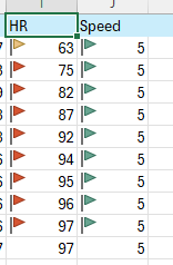
We can understand from above picture that for a given speed,
we have more number of cases with increased HR.
3.Highlighting text that contains specific keywords: Use “Highlight Cells Rules” with the “Text that Contains” option to flag cells or “Format cells based on their values” with particular values.
From this data, we can analyze that male % is > than female%.

Duplicate Values: There is one of the options for the condition, and can check for both duplicate and unique values.
Here is the Highlight Cell Rules part of the conditional formatting menu:

Select the range, Click on the Conditional Formatting icon and Select Duplicate Value from the dropdown menu. Select the appearance option “Yellow Fill with Dark Yellow Text” from the dropdown menu

We can see the duplicate values are highlighted.
Top 10/ Bottom 10 rules:
Top/Bottom Rules are premade types of conditional formatting in Excel used to change the appearance of cells in a range based on your specified conditions.
Here is the Top/Bottom Rules part of the conditional formatting menu:

The “Top 10 Items” or “Bottom 10 Items” rules will highlight cells with one of the appearance options based on the cell value being the top or bottom values in a range.

Now, We can identify the top 10 Heart rate (HR) values with their IDs.
4. Tips for Effective Use:
Use clear and concise rules:
Define rules that are easy to understand and that accurately reflect what you want to highlight.
Choose appropriate formatting:
Select colors, icons, or styles that are visually distinct and easy to interpret.
Test your rules:
Preview the conditional formatting before applying it to ensure it highlights the data you intend to highlight.
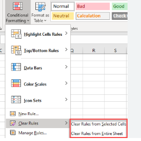
Clear Formatting:
Navigate to the “Home” tab, click the “Clear” dropdown, and choose “Clear Formats”. This will remove all formatting from the selected cells, leaving only the content and any comments.
What are Absolute and Relative References?
In Excel, relative references adjust automatically when you copy or drag a formula to a new cell, reflecting the new cell’s position. Absolute references, on the other hand, remain constant regardless of where the formula is copied, always referring to the same cell.
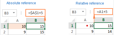
If you're checking whether values in each row meet a condition compared to a specific cell, use absolute references.
If you're comparing each cell to itself or to another in the same row/column, use relative references.
When using formulas in conditional formatting, be mindful when using absolute references (e.g., $A$1) to avoid issues with the formula changing as it’s applied to different cells.
Conclusion:
Conditional formatting in Excel allows users to automatically highlight or modify the appearance of cells based on predefined conditions, making data analysis and presentation more intuitive and efficient. It also helps in automated formatting and makes it easier to manage as we can customize the formatting rules.
Happy exploring!


