PIVOT TABLE AND VISUALIZATION IN EXCEL
Pivot tables are one of the most powerful and useful features in Excel. With very little effort, you can use a pivot table to build good-looking reports for large data sets. Pivot tables can dramatically increase your efficiency in Excel.
What is a Pivot Table:-
A PivotTable is an interactive way to quickly summarize large amounts of data. You can use a PivotTable to analyze numerical data in detail, and answer unanticipated questions about your data. A PivotTable is especially designed for:
Present large amounts of data in a user-friendly way.
Summarize data by categories and subcategories.
Filter, group, sort and conditionally format different subsets of data so that you can focus on the most relevant information.
Rotate rows to columns or columns to rows (which is called "pivoting") to view different summaries of the source data.
Subtotal and aggregate numeric data in the spreadsheet.
Expand or collapse the levels of data and drill down to see the details behind any total.
Present concise and attractive online of your data or printed reports.
For example, here's a simple list of Sales data in the below table , and a PivotTable based on the list next to it.

Sales data | Corresponding PivotTable |

How to create a Pivot Table :-
Step 1: Find Your Source Data
Before you can make a pivot table, you need to get all your information organized in an Excel spreadsheet.
So, the first step is to figure out what the source of your data is.
Step 2: Import Data Into Excel
To save some time and to maximize productivity, you can import data to an Excel spreadsheet. Here’s how:
Open a new Excel spreadsheet, then select the “Data” tab at the top.
Select the import option that fits your data. Your data is probably in a CSV or HTML file format, but all of the choices are a possibility depending on the platform or software you’re using.
For example, if you are uploading data from a CSV file, you’d select “From Text.”

You can also select “From other sources” if you need to upload data from an SQL server or other sources.
Step 3: Clean Up Your Imported Data
While Excel is extremely useful, it’s not always flawless. It's possible that your import process didn’t go 100-percent perfect. Take some time to go through your information and fine-tune any incorrect fields.
For example, columns that are supposed to be a currency, such as USD, may appear as regular numbers.
Just highlight the cells and select your currency under the “Number” section on the “Home” tab.

There could be some other minor import problems, but it’s nothing you can’t sort out quickly. It’s important to get all your data organized before you attempt to create a pivot table. Make sure your source table contains no blank rows or columns, and no subtotals.Using an Excel Table for the source data gives you a very nice benefit - your data range becomes "dynamic". In this context, a dynamic range means that your table will automatically expand and shrink as you add or remove entries, so won't have to worry that your Pivot Table is missing the latest data.
Step 4: Create a Pivot Table
You don’t need to select the entire spreadsheet to create a pivot table. Just go with the required fields., and then go to the Insert tab > Tables group > PivotTable.

This will open the Create PivotTable window. Make sure the correct table or range of cells is highlighted in the Table/Range field. Then choose the target location for your Excel Pivot Table:
Selecting New Worksheet will place a table in a new worksheet starting at cell A1.
Selecting Existing Worksheet will place your table at the specified location in an existing worksheet. In the Location box, click the Collapse Dialog button to choose the first cell where you want to position your table.

Clicking OK creates a blank Pivot Table in the target location, which will look similar to this:

5.Arrange the layout of your Pivot Table report:-
The area where you work with the fields of your summary report is called PivotTable Field List. It is located in the right-hand part of the worksheet and divided into the header and body sections:
The Field Section contains the names of the fields that you can add to your table. The filed names correspond to the column names of your source table.
The Layout Section contains the Report Filter area, Column Labels, Row Labels area, and the Values area. Here you can arrange and re-arrange the fields of your table.

The changes that you make in the PivotTable Field List are immediately reflected to your table.
6. How to add a field to Pivot Table
To add a field to the Layout section, select the check box next to the field name in the Field section.
By default, Microsoft Excel adds the fields to the Layout section in the following way:
Non-numeric fields are added to the Row Labels area;
Numeric fields are added to the Values area;
Online Analytical Processing (OLAP) date and time hierarchies are added to the Column Labels area.
7.How to arrange Pivot Table fields
You can arrange the fields in the Layout section in three ways:
1. Drag and drop fields between the 4 areas of the Layout section using the mouse. Alternatively, click and hold the field name in the Field section, and then drag it to an area in the Layout section - this will remove the field from the current area in the Layout section and place it in the new area.
Right-click the field name in the Field section, and then select the area where you want to add it:

Click on the filed in the Layout section to select it. This will also display the options available for that particular field.

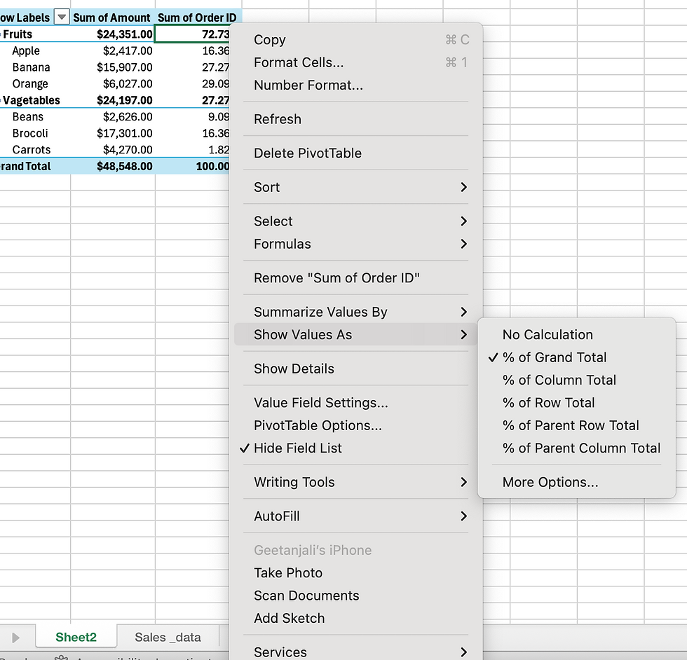
8.Show different calculations in value fields (optional)
Excel Pivot Tables provide one more useful feature that enables you to present values in different ways, for example show totals as percentage or rank values from smallest to largest and vice versa. The full list of calculation options we can see it in the following picture.
This is how you create Pivot Tables in Excel.
You can use a PivotTable to summarize, analyze, explore, and present summary data. PivotCharts complement PivotTables by adding visualizations to the summary data in a PivotTable, and allow you to easily see comparisons, patterns, and trends. Both PivotTables and PivotCharts enable you to make informed decisions about critical data.
PivotCharts provide graphical representations of the data in their associated PivotTables. PivotCharts are also interactive. When you create a PivotChart, the PivotChart Filter Pane appears. You can use this filter pane to sort and filter the PivotChart's underlying data. Changes that you make to the layout and data in an associated PivotTable are immediately reflected in the layout and data in the PivotChart and vice versa.
PivotCharts display data series, categories, data markers, and axes just as standard charts do. You can also change the chart type and other options such as the titles, the legend placement, the data labels, the chart location, and so on.
CREATE A PIVOT CHART
To keep things simple, we will continue with the same example that we used earlier.
Click any Cell in Your Pivot Table . It doesn’t matter if it’s a word, number, total, or header. Just make sure a cell within the table is highlighted.
Go to the "Pivot Table Analyze"tab in the Top Ribbon .

Then click on the PivotChart icon. I have selected a 3D-pie chart for visualization.

CONCLUSION:-
PivotTable and PivotChart provide a clear and concise summary of data, allowing users to identify trends, patterns, and insights more easily than in raw data. They are powerful tools for data analysis and visualization, making it easier to understand complex information and make informed decisions.


