Excel for Beginners - The Basics

As big data continues to change the way businesses operate and drive strategy, the ability to efficiently and effectively organize and analyze data is crucial. Managers need to be able to utilize tools to identify trends and help make better business decisions. Microsoft's Excel is a powerful spreadsheet software to organize and manage data related to business operations. This blog focuses on mastering the fundamental tasks performed in Excel, including data entry, basic formula calculations, and functional operations.
The Anatomy/Layout of the Spreadsheet:
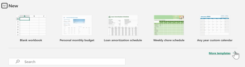
To open a new worksheet, you can allows go to New Workbook or you can also try different templates by clicking More Templates or even you can search for a different template.
A blank Workbook will always have one sheet open; you can relatively have more sheets to work on. The sheets all together is called the Workbook
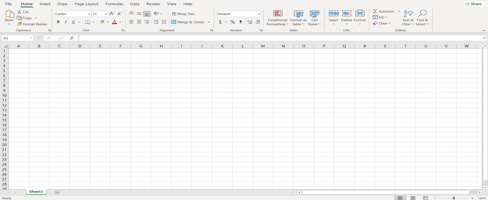
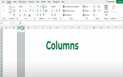
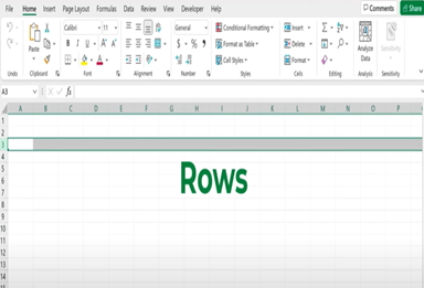
Each Spreadsheet will have a Column and a Row. Every column has a column letter and every row has a row number. The intersection of column and a row is the cell.
An excel sheet may contain 17 billion cells. When you click on a cell, it becomes an active cell.
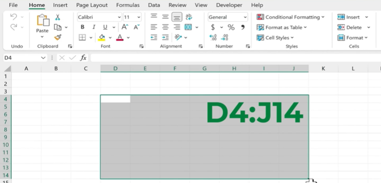
A Range: It is a collection of cells that is generally grouped together.
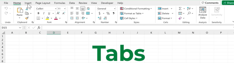
Tabs: In addition to the anatomy of the spreadsheet we also need to learn about the layout we are going to work with. The layout starts with the Home button, followed by Insert, Page Layout. etc.
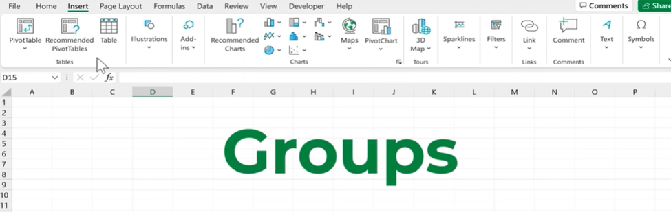
Ribbon: Whenever you click a tab the tools button below here changes and this part of the layout is called Ribbon.

Group: Each Ribbon is divided into groups, like below the Tables group, the charts group. Each of them is divided by a line.
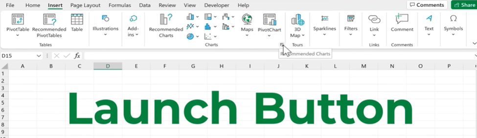
Not all of the options can fit in such groups. For example, the charts group is not big enough to hold all of the options. So some of the groups will have to expand when you click the small icon in the ribbon called the Launch button.
When you click on the Launch Button or also called a Dialogue Box Launcher. The box opens up more clearly, this shows the icons that doesn’t fit inside the Ribbon.
· In addition to Tabs, Ribbons, Launch Buttons there is also Up and down Horizontal and Vertical Scroll Bar. We can have a Zoom in and Out option on the bottom right corner of the spreadsheet.
· There are also view button on the bottom right corner: Normal, Page Layout and Page Break Preview. Most of us work on the Normal View on our daily workflow.
On the Top Left corner, we can see the Name box where we see which cell is selected/used.

Now, we also see the very top bar of our Excel where there is Quick Access Tool Bar. We can customize our quick Access toolbar according to our need and comfort.
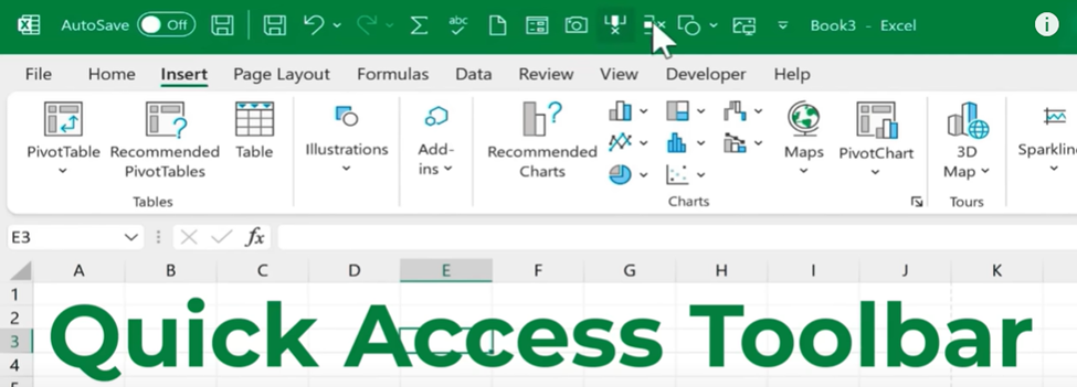
The Center in that bar gives you the name of the workbook and the right top corner is where you see a X mark to close the workbook.
We can see an interesting space above the work sheet is called the Formula Bar. This is where we go to enter formulas in you excel spreadsheet.

Now that we know the Anatomy and Layout of the worksheet. We are completely ready to begin learning to use Excel.
We will begin by saving this workbook. For that we have to click the File on the left top corner, first it will ask you use Save As, I that you can decide where to Save your workbook. Document folder -> Excel for Beginners -> SAVE.
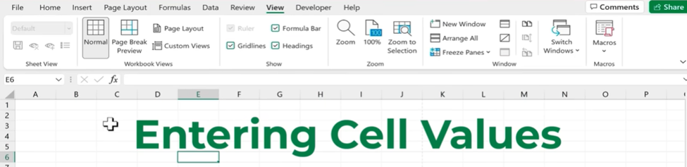
Now Let’s begin by adding cell values for the worksheet.
Let's take an example, we work for a small business and they are asking us to create a payroll spreadsheet.
Column A: Employee ID numbers
Column B: Employee Names
Column C: Wages
Anytime to enter data in excel you have to select that cell. There is a saying ‘Select to Affect’, you have to select that cell to affect that cell.
Now that we start entering the cells. You type 1 for Employee ID, then hit Enter – It goes to the next cell. Then type 2 Enter, 3 Enter, 4 Enter, 5 Enter and So on...
For this kind of filling Microsoft excel has brought in some feature call Fill Handle or Auto Fill Handle.
The Auto Fill Handle will identify the pattern and help you fill the consecutive cells. You have to just select the range of cells, there will be a small + sign at the bottom of the box. You have to just drag and drop wherever needed.

To Edit any cell, you can just double click on the cell and go rewrite or correct that particular cell alone and the click ENTER to save the changes and move you to the next cell.
Short- Cuts:
To move down a cell we use ENTER, to move UP a cell we use SHIFT+ENTER.
If we press TAB, we move to the right-side cell and SHIFT+TAB to move to the left-side cell.
To Copy Paste we use the easiest way CTRL+C and CTRL+V to copy cell values and paste.
To UNDO a cell or any work in the worksheet we use CTRL+Z.
To Delete a Cell, you can either use the DELETE button and double click and use backspace or you can go to HOME tab and on the right side you have this option shown below. If you use Clear All you can clearly delete all the content/formula associated with that particular cell.

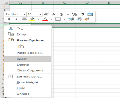
INSERT: To Insert any Row/Column you can just right click on any Row/Column and click Insert
FIT CHECK: To fit any values inside a cell you can simply keep your cursor in between the column and drag or double to fit into its size.

This can be done for the entire range, if you want to double click between column letter for that entire range, it will adjust all the cells in the selected range to fit into the cell.
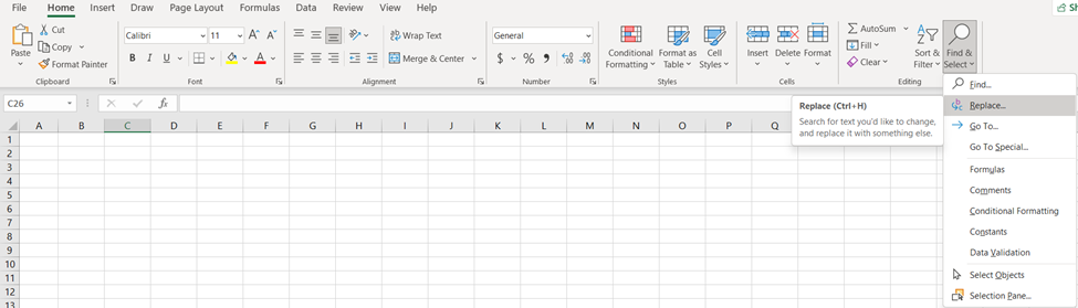
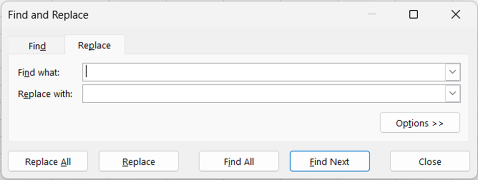
FIND and REPLACE: Short cut (CTRL+H) If you want to find any values and replace them, you can hit the HOME tab and go to this magnifying glass. Select FIND or REPLACE and update the worksheet.
AUTO – CORRECT Features:
You can explore various Auto Correct options in Excel, go to FILE -> Options -> Proofing ->AutoCorrect Options.
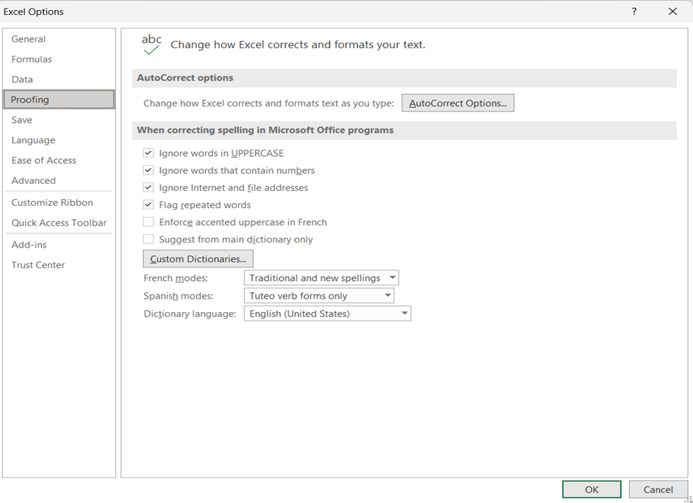
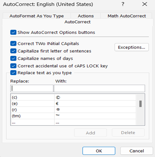
We can make alterations to the already exists auto correction or we can customize/add auto corrections and adjust them to our advantage.
MOVE the contents of the cell: Select the cell you want to move, now you see a cross bar on the outline of the cell, you click and drag the cell to a different location.
We can do the same for a Range. Select the range and go to the very edge of the range, Select and drag to the desired location.
Errors in Excel: From time to time you may make mistakes in excel. For example if type an incorrect formula the excel will give an error message when you hit Enter.
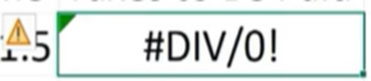
Or sometime we receive a warning saying your formula was incorrect, do you want excel to give you suggestions.
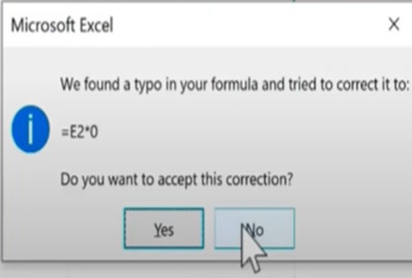
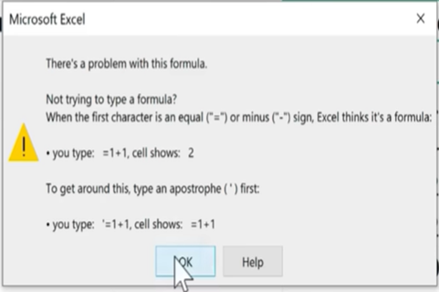
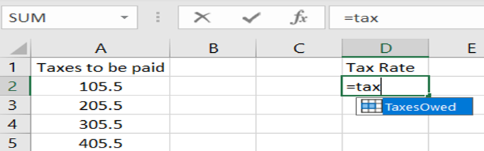
Change the Name: It is important to know that in Excel we can change the name of the cell or the name of a range. If we select the particular cell or the range and go to name bar and change the name and hit Enter. Now that range will have its own special name.
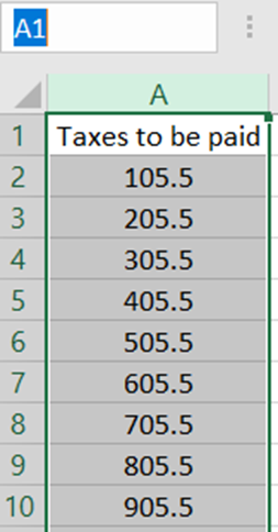

If we forget the name of that range, we can always go and check the name bar to check.
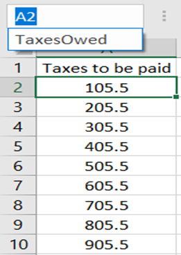
Where will the naming be used in Excel, instead of referring just to a cell we could refer to the name of the cell ‘TaxesOwed’.
FORMULAS
Excel is a spreadsheet tool, YES but it is also a calculator. It has several built-in calculator functions and operators that we would need.
In Excel whenever you start creating a formula you should start with ‘=’.
To start with, we first have to select the cell we are going to create the formula and use accordingly. For example, we are creating taxable income for employees, we calculate hourly wage X hours worked. Here in excel we use * for multiplication.
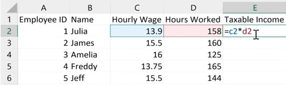
To fill the rest of the employee’s taxable income in the column you just have to double click on cell E2, it auto fills the rest of the employee wages.
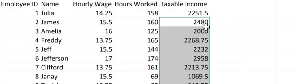
In excel anytime to extend a formula or work on a formula it is always easy to use the formula bar on the left side above the spread sheet.
Relative cell reference in Excel: By default, a cell reference is a relative reference, which means that the reference is relative to the location of the cell.
As an example, if you copy the formula =B4*C4 from cell D4 to D5, the formula in D5 adjusts to the right by one column and becomes =B5*C5. If you want to maintain the original cell reference in this example when you copy it, you make the cell reference absolute by preceding the columns (B and C) and row (2) with a dollar sign ($). Then, when you copy the formula =$B$4*$C$4 from D4 to D5, the formula stays exactly the same.

Absolute and Mixed reference: Less often, you might want to mix absolute and relative cell references by preceding either the column or the row value with a dollar sign ($)—which fixes either the column or the row (for example, $B4 or C$4).
To change the type of cell reference:
1. Select the cell that contains the formula.
2. In the formula bar , select the reference that you want to change.
3. Press F4 to switch between the reference types.
The table below summarizes how a reference type updates if a formula containing the reference is copied two cells down and two cells to the right.
For a formula being copied: | If the reference is: | It changes to: |
$A$1 (absolute column and absolute row) | $A$1 (the reference is absolute) | |
A$1 (relative column and absolute row) | C$1 (the reference is mixed) | |
$A1 (absolute column and relative row) | $A3 (the reference is mixed) | |
A1 (relative column and relative row) | C3 (the reference is relative) |
FUNCTIONS
Functions are predefined formulas that perform calculations by using specific values, called arguments, in a particular order, or structure. Functions can be used to perform simple or complex calculations. You can find all of Excel's functions on the Formulas tab on the Ribbon: Excel function syntax.
A Formula is an equation designed by a user in Excel, while a Function is a predefined calculation in the spreadsheet application.
I) Basic Excel Functions and Formulas
1. SUM Function
2. Average Function
3. COUNT Function
4. COUNTA Function
5. MAX and MIN Function
6. ROUND Function
7. TRUNK Function
8. MEDIAN Function
9. Function
10. LEN Function
Basic Excel Functions and Formulas
In Microsoft Excel, Formulas and Functions are integral components for performing calculations and data analysis. Formulas are user-defined expressions that execute calculations by combining mathematical operations, cell references, and Functions. For example, a Formula like "=A1+B1" adds the values in cells A1 and B1.
On the other hand, Functions are pre-built operations designed to simplify complex tasks, offering efficiency in spreadsheet calculations. An illustration of this is the SUM Function, which adds up values in a specified range, such as "=SUM (A1:A5)," summing the values in cells A1 through A5.
In essence, Formulas and Functions empower users to automate computations, manipulate data, and streamline the analytical processes within Excel. Let's look at the top 14 Basic Excel Functions:
1) SUM Function
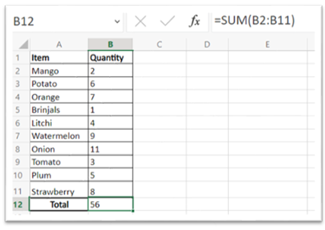
The SUM Function in Excel adds values in one or more cells or all the values in a cell range. The syntax for SUM Function starts with an equal (=) sign, then the functions name SUM and you have to include cell reference or range in each argument.
In the example give below, we are adding the quantity of all items in the cell range B2 to B11, where B is the column, and 2 and 11 is the row number in the B column. Select the cell where you need the answer and type the formula =SUM (B2:B11).
2) Average Function
As the Function's name indicates, AVERAGE Functions is used to find the average values in two or more cells or a cell range. The syntax is similar to the SUM Function, starting with the equal sign (=) sign and then AVERAGE and cell reference.
For example – In the same table, to find the average of all quantity values between B2 to B11, select all the values between the 2nd and 11th row in the B column to find the average.
3) COUNT Function
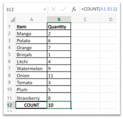
Let's say in an extensive data set; you need to find how many cells contain numeric values, then you can use the COUNT Function. This function will make this significantly easier for you than manually counting all the cells. This Function also starts with = sign, function name – COUNT and then the cell reference in arguments. In the image below we will find how many cells between A1 to B11 contain numeric values.
4) COUNTA Function
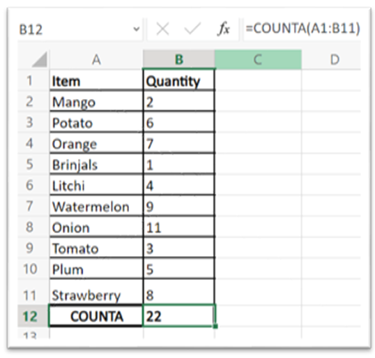
Like the COUNT Function, this function will count how many cells contain any values. These values can be numeric or alphabetical.
For example, in the table given below we are finding how many cells between A1 and B11 contain values using =COUNTA(A1:B11).
5) MAX and MIN Function
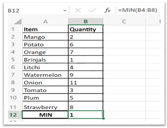
MAX Function can be used to find the maximum value in a range of cells, and the same goes with MIN Function. The syntax for MAX and MIN Functions starts with = sign, function name, and cell reference.
For example, you can find the maximum and minimum value between B4 to B8 using =MAX (B4:B8) and =MIN (B4:B8)
a) MAX Function
Here's how MAX Function works in Excel:

b) MIN Function
Here's how MIN Function works in Excel:
6) ROUND Function
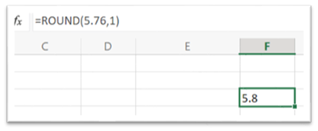
The ROUND Function can be used to round off a decimal number in your data in Excel. The syntax starts with = sign, function name and then the number you want to round off. For example, using the following formula to round off 5.76 to one decimal place.
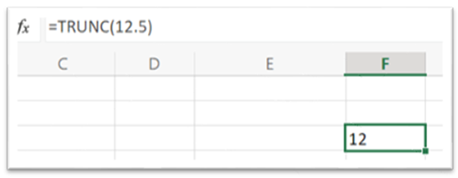
7) TRUNC Function
As the name suggests, TRUNC Function is used to truncate numbers. You can use this Function to remove decimals from the number instead of rounding it. The syntax starts with = sign, function name and then enter the digits in the brackets. In the following image truncated 12.5. So, the result will be the number 12, eliminating the digits after decimals. Use the syntax =TRUNC (12.5) in your sheet.
8) MEDIAN Function
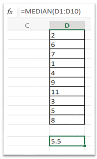
If you want to know the middle value between the maximum value and minimum value in the data set, use the MEDIAN Function. The syntax order is similar, starting with an equal (=) sign, Function name, and cell reference. This Function will give you the middle value in the cell range.
To find the middlemost value between the maximum and minimum value in our data by use =MEDIAN (D1:D10).
9) IF Function
IF Function is used to perform a logical test in Excel. The IF Function checks if a condition is met and gives one value if the result is true or false.
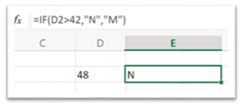
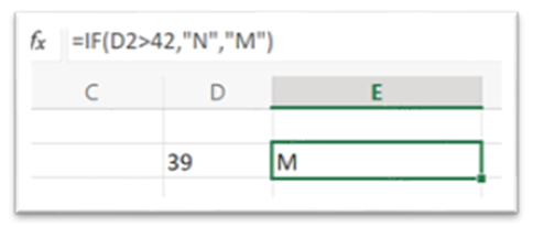
For example – in the following image, we are checking if the number in the D2 cell is greater or smaller than 42. If the number in D2 is greater, we will get the result as ‘N’, and if it is not, we will get the result as ‘M’.
For example - Here we are considering the number 48, which is greater than 42, we will use =IF(D2>42,"N","M") and get the result as ‘N’.
Now, we will consider the number 39, smaller than 42. We should get the result as ‘M’, which is the value for false. This fails the logical test.
10) LEN Function
This Function counts the length of characters in a cell or cell range. Remember that even the spaces between the letters are counted as characters.
For example – First, let's see how LEN Function works in a single cell.
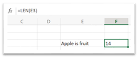
Now, let's see a range of cells. Here the syntax will remain the same we will only give the complete cell range details.
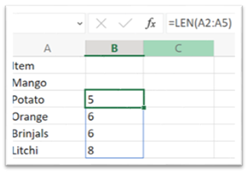
You can use the complete cell range or just the fill handle to get the characters of data below the one already found.
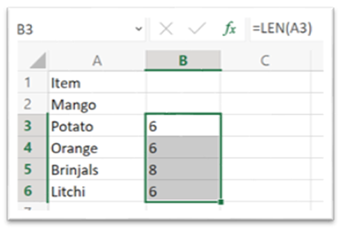
NOW Function
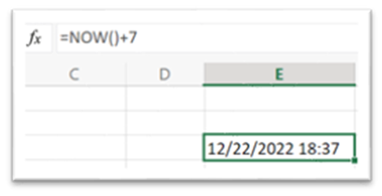
If you have wanted to write the current time or date in your spreadsheet, the easiest way is to use the NOW Function. Just put the syntax =NOW(), and you will have the exact date and time. If you want to move a few days ahead and check the date, add that many numbers to the syntax. For example, for today’s date and time use the following syntax:
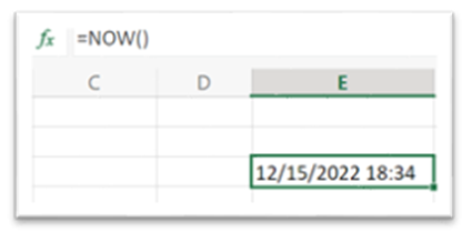
If you have to see the date seven days later, just type =NOW ()+7
12) TRIM Function
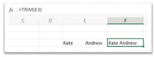
If you have copied something and pasted it into an Excel cell, you would have noticed it contains extra spaces. If you want to eliminate these spaces between text, you can use the TRIM Function. The syntax for TRIM Function is =TRIM(cell reference)
Here's how you can eliminate the extra space between Kate and Andrew:
13) PRODUCT Function
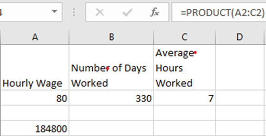
The PRODUCT Function helps us in case we need to multiply the values in two or more cells. Just put the syntax as PRODUCT(value1, value2,...) in order to use the function. For example – if you are looking to calculate Andrew’s yearly income based on his hourly wage, use this formula:
14) COLUMN and ROW Function
The COLUMN Function returns the column number of a given cell reference. For example, the formula =COLUMN(A1) return the value 1 since Column A is the first column in the spreadsheet.
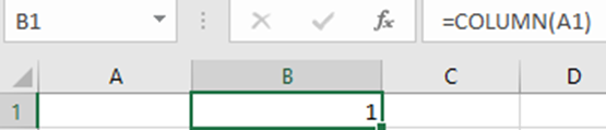
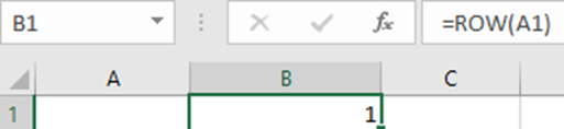
Similarly, the ROW Function returns the row number of a given cell range. For example, the formula =ROW(A1) returns the value 1 since Row A is the first row in the spreadsheet.
Conclusion
The Basic Excel Layout, Formulas and Functions discussed in this blog will help you succeed in any profession. Learning Excel is always a good use of time, as you only get more proficient at completing your tasks faster. If you’re interested in a job role that deals with data and calculation, you must learn to use these Excel functions. Understanding the difference between Function and Formula in Excel can greatly enhance your ability to analyze and manipulate data effectively.


