Descriptive Statistics and Beyond: A Clinical SAS Programmer’s Journey into PostgreSQL

Introduction: The Analytical Pivot

In my previous post, we treated the Student Performance Dataset like a digital training ground. We focused on the "how" of data cleaning—scrubbing text, fixing nulls, and standardizing schemas. It was the perfect exercise for a data "workbench" setup.

However, as a former Clinical SAS Programmer, I know that cleaning is only half the battle. The true value of a database isn't just in its cleanliness; it’s in its ability to act as an analytical engine. To demonstrate this, I’ve decided to move away from the student data and pivot to a more complex, high-stakes domain: The Heart Disease UCI Dataset.

Why the Switch?

While the student data was great for practicing "standardization," clinical data requires validation. In clinical programming, we are used to the “Extract, Load, Analyze” workflow—pulling data out of a database to run it through SAS PROCs. But why pay the "Data Tax"?

The "Data Tax" is that hidden cost of time and resources spent moving large files between environments. By switching to the Heart Disease dataset, I can show you how to perform a full statistical workup—from descriptive statistics to predictive modeling—directly inside PostgreSQL.

We aren't just cleaning anymore; we are performing a clinical investigation where the data lives.

Phase 1: Infrastructure and Ingestion

Step1: Establishing the Clinical Library

In SAS, we define libraries. In PostgreSQL, we define Tables with Strict Schemas. This is our "Data Contract." By defining the types (INT, NUMERIC) upfront, we ensure that clinical values like Blood Pressure and Cholesterol are valid before the analysis even starts.

Defining a table

Step 2: Getting data into pgadmin

I followed the standard steps to import a CSV file into pgAdmin. Please refer to my previous blog for the steps to be taken. To ensure the data was imported correctly, I used a LIMIT 5 query as a quick check.

To ensure if the data is imported.

Phase 2: Clinical Validation and Discovery

Step3: Descriptive Statistics (The "PROC MEANS")

The first step is checking the "Center" of the data. I want to see how clinical markers differ between my cohorts to ensure the data is logically sound.

The Insight: I use AVG() and STDDEV() to look at the Maximum Heart Rate achieved (thalach).

The Finding: The SQL output shows that Target 1 has a significantly higher cardiac reserve (158.47 bpm) compared to Target 0 (139.10 bpm).

Step4: Clinical Validation (The Reality Check)

In clinical trials, we never trust labels blindly. I ran a cross-check on Oldpeak (ST depression), a measure used in EKGs where higher values traditionally indicate heart disease.

The Result: Target 0: 1.58 (Higher stress indicator)

Target 1: 0.58 (Normal range)

This confirms that in my specific dataset, Target 0 is the Disease group and Target 1 is the Healthy group. Seeing this immediately in pgAdmin validates the integrity of my library before I ever move to a reporting tool.

Phase 3: Patterns and Distributions

Step5: Visualizing with the Console Histogram:

A standout feature in Postgres is the width_bucket() function. It allowed me to create a "Console Histogram" to visualize the distribution of Cholesterol (chol) across my patients without needing any external software.

The Insight: By grouping cholesterol into specific ranges, I can see exactly where the bulk of my population lies. For instance, my results show that the largest group of patients (186 individuals) falls within the 208 to 296 mg/dl range.

repeat ('■', ...): "We are essentially telling SQL to draw a bar chart using text characters, scaling the length of the bar based on the patient count in that bucket."

Step6: Risk Correlation (PROC CORR)

In clinical trials, risks rarely exist in isolation. I used the CORR() function to calculate the Pearson Coefficient between Age and clinical markers like Cholesterol and Blood Pressure.

The Finding: The positive correlation (0.21 for cholesterol and 0.28 for blood pressure) confirms that as the population ages, these risk markers trend upward. It proves the database can handle complex math—like correlation—in milliseconds.

Phase 4: Advanced Modeling and Stratification

Step7: Predictive Analytics and Statistical Dependence

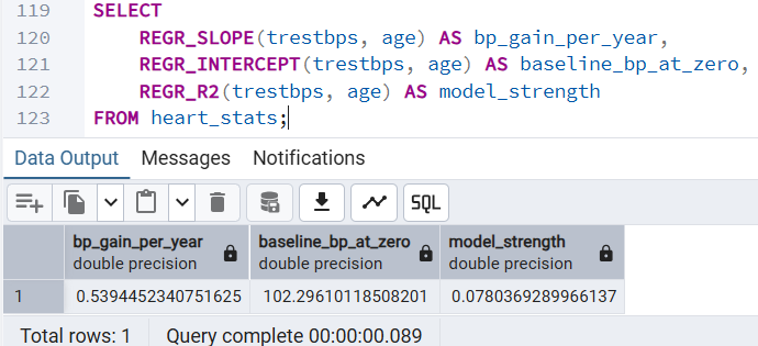
One of the most powerful realizations was that SQL can predict. I used REGR_SLOPE to calculate the "Baseline of Aging"—predicting how much Resting Blood Pressure increases per year of age.

The Insight: The slope (0.539) tells us exactly how many units of blood pressure a person typically gains per year of life in this cohort.

The Finding: This allows us to move from "describing" the past to identifying patients whose BP is abnormally high for their specific age group.

Step8: Risk Stratification: Identifying High-Risk Outliers

In clinical work, we are often tasked with identifying the "extremes" within a population. Using the NTILE(10) window function, I was able to partition the dataset into deciles without collapsing the individual rows.

The Insight: This analysis allowed me to isolate the top 10% of patients based on serum cholesterol levels. The Finding: This instantly identifies high-priority individuals, such as the 67-year-old patient with a cholesterol level of 564 mg/dl, who may require immediate clinical intervention.

Step9: Categorical Analysis: Heart Disease Prevalence by Age

Transitioning a continuous variable like Age into discrete "Risk Groups" is the PostgreSQL equivalent of a SAS FORMAT. This allows us to see how disease prevalence shifts across different life stages.

The Insight: I used a CASE statement to categorize patients into 'Young', 'Middle-Aged', and 'Senior' buckets. The Finding: Surprisingly, in this specific dataset, the 'Young' group (<45) showed the highest disease prevalence at 75%. This type of automated stratification is essential for identifying unexpected trends in a clinical population.

Step10: Variance Analysis: BP Consistency Across Pain Types

Averages often hide the truth; we need to understand the "spread" of the data to identify clinical variability. Using the VARIANCE() and STDDEV() functions, I analyzed Resting Blood Pressure across different Chest Pain categories.

• The Insight: Comparing how much blood pressure fluctuates based on the type of chest pain reported.

• The Finding: High variance in a specific category suggests a heterogeneous group. This indicates that patients within that chest pain type may have vastly different underlying conditions, requiring more granular investigation than a simple mean would suggest.

Step11. Individual Patient Percentile Ranking

Finally, I used the CUME_DIST() window function to calculate the Percentile Rank for each patient’s cholesterol.

• The Finding: Identifying "clinical outliers" in the highest percentiles (99th-100th percentile) provides a much clearer signal for intervention than just looking at raw numeric values.

To wrap things up, I’ve put together a quick-reference guide for my fellow SAS programmers. Transitioning to PostgreSQL doesn't mean learning statistics all over again; it simply means learning a new way to call the same powerful mathematical engines we've always relied on. Here is how the most common SAS Procedures translate directly into PostgreSQL functions within pgAdmin:

SAS Procedure	PostgreSQL Equivalent	Clinical Utility
PROC MEANS	AVG(), STDDEV(), VARIANCE()	Basic cohort baselines
PROC CORR	CORR(x, y)	Identifying linked risk factors
PROC REG	REGR_SLOPE(), REGR_INTERCEPT()	Trend prediction and aging models
PROC RANK	NTILE(), CUME_DIST()	Identifying outlier patients
PROC FORMAT	CASE WHEN... THEN	Patient stratification (Risk Groups)

My perspective as a programmer is this: PostgreSQL removes the "Data Tax." I no longer spend time moving data back and forth between tools for initial discovery. By doing the math where the data lives, I have gained a deeper respect for the database as an analytical engine and a clearer understanding of the clinical data itself.

I hope this walkthrough has highlighted some powerful functions you might not have explored yet!

Which SAS procedure will you try to replace in pgAdmin today? 😊