Data Cleaning and SQL Query Setup in PostgreSQL
Updated: Jan 15
Data cleaning is the process of fixing or removing data that's inaccurate, duplicated, or outside the scope of your research question. Some errors might be hard to avoid.
Why we need to clean Data?
may receive messy data from clients which require data cleaning to make sure correcting errors and inconsistencies in raw data sets to improve data quality. This is called as Data cleaning, also called data cleansing or data scrubbing.
What happens it data not cleaned?
If data not cleaned, dirty data may lead to incorrect beliefs and assumptions about data-driven insights, poorly informed decisions based on those insights and distrust in the analytics process overall.
Challenges
Data Integration: Combining data from multiple wearables and sources with different formats and timestamps.
Data Quality Issues: Handling missing, noisy, or inconsistent readings from sensors.
Complex Querying: Managing large datasets efficiently and writing optimized SQL queries for time-series data.
Feature Extraction: Identifying meaningful metrics (e.g., glucose variability, EDA peaks) from continuous signals.
Privacy & Ethics: Ensuring sensitive health data is securely stored and anonymized.
Learnings
Gained hands-on experience with real-world biomedical and wearable datasets.
Improved data cleaning, transformation, and analysis skills using SQL and Python.
Understood the importance of temporal data alignment across multiple devices.
Learned to translate physiological data into clinical insights and behavioral patterns.
Enhanced problem-solving through data-driven exploration and visualization.
Project Details
The Glycemic Variability project focuses on analyzing patient-level data to better understand fluctuations in glucose levels and their relationships with physiological measurements and dietary intake. The dataset includes multiple tables capturing patient demographics, heart rate, inter-beat intervals, continuous glucose monitoring data, skin temperature, electrodermal activity, and food intake logs. To ensure accurate analysis, a comprehensive data cleaning and transformation process was performed. The cleaned datasets are now consistent, reliable, and ready for predictive analysis, providing a solid foundation for insights into glycemic variability patterns.
Data Backup
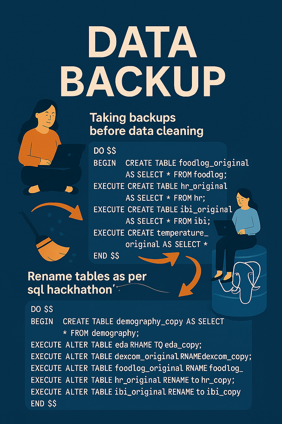
Data backup protects your original datasets before any cleaning or transformation, ensuring nothing is lost or overwritten. It allows you to revert to the raw source if errors occur during processing. Backups also support audit trails and reproducibility in clinical and analytics workflows.
In SQL hackathons or production systems, It is best practice they’re essential for safe experimentation and reliable query development.
After working on data backup, you can compare the tables with original tables from given data.
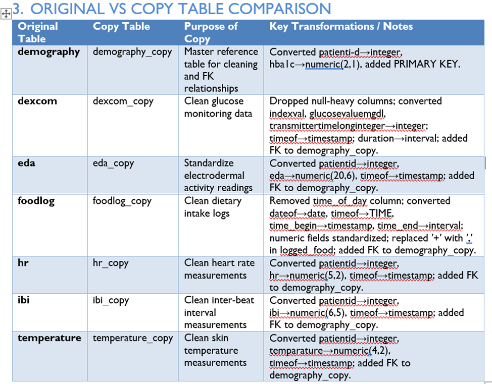
DATABASE CLEANING & TRANSFORMATION OVERVIEW

The Glycemic Variability Database consists of seven main tables Copies of all tables (demography_copy) were created to preserve the original data while applying cleaning and transformation operations Each table stores different types of information and is linked to the demography table through the patient-id field to maintain referential integrity. All work was performed on copied tables (e.g., demography\_copy),leaving the original source data untouched.
Relationships in GVDatabase
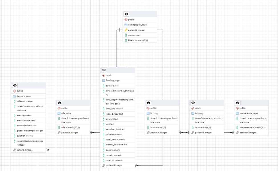
Data Relationships – v Foreign Key Relationships: All demography_copy tables link to demography_copy through the patient-id field.
v Integrity Constraints: Primary keys were added to demography_copy, and foreign keys were applied to other tables to enforce data consistency.
v Purpose of Copies: Creating _copy tables allow safe transformations and data cleaning without modifying the original tables.
Key Observations –
-> Column data types were standardized
-> Null and duplicate values were identified and removed where necessary.
->Unnecessary columns were dropped from tables like dexcom_copy and foodlog_copy.
-> All cleaned tables are now ready for analysis, with consistent formats and reliable relationships across datasets.
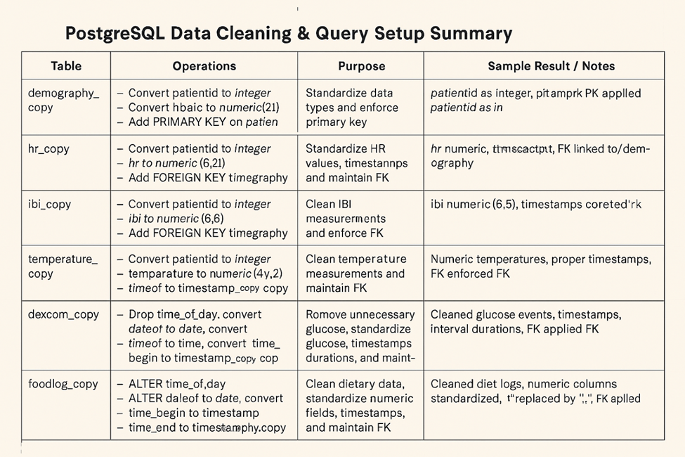
Here is the summary for the data cleaning and query setup details for the tables after data cleansing.
ER Diagram for the Glycemic Variability data
What is Query?
Query is a declarative SQL statement used to retrieve, insert, modify, or delete data within a database. It functions as a request or command for the database management system to perform a specific action and return the results in the form of a result set (a virtual table). :
How to write Queries?
.
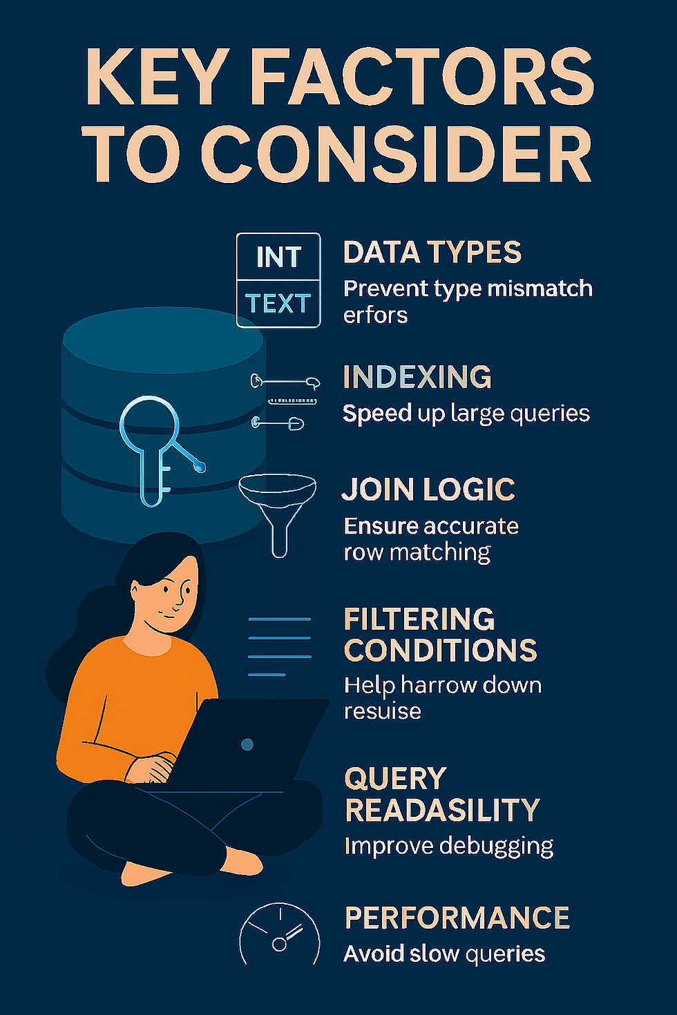
Writing queries in SQL/PostgreSQL, uses a language called SQL (Structured Query Language), which focuses on telling the data base what data you want to display.
Here I want to share few queries that I choose while selecting categories with reasons
It pulls temperature readings from the temperature_copy table and displays them in reverse chronological order — so the most recent measurements appear at the top.
Question 1: 1 What is the average glucose level during meal windows?
QUERY – SELECT f.logged_food, AVG(d.glucosevaluemgdl) AS avg_glucoseFROM Dexcom dJOIN foodlog f ON d.timeof BETWEEN f.time_begin AND f.time_endGROUP BY f.logged_food;
Now lets breakdown this query:
What the Query Does
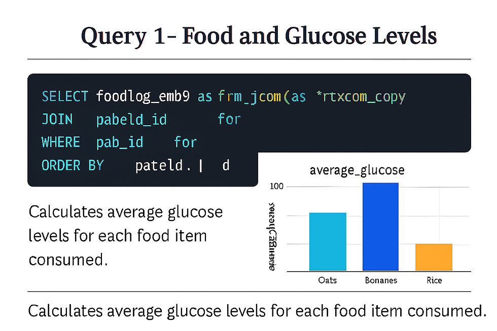
Links glucose readings to food events
It matches each glucose measurement (Dexcom) to the food item logged in foodlog based on timestamp overlap.
Uses a time-window join
d.timeof BETWEEN f.time_begin AND f.time_end ensures that only glucose values occurring during the food’s digestion window are included.
Aggregates glucose response by food type
AVG(d.glucosevaluemgdl) gives the mean glucose level associated with each food item.
QUERY
Question2: About Food Consumption Time Ranges
Query SELECT
patientid,
logged_food,
tsrange(time_begin,time_begin+time_end,'[)') AS meal_time_range
FROM foodlog_copy;

Breakdown of the Query:
Creates a PostgreSQL range type (tsrange) representing the time window of a meal.
Uses:
time_begin → start of the meal
time_begin + time_end → end of the meal (assuming time_end is a duration)
The '[)' notation means:
Inclusive of the start time
Exclusive of the end time
Range types allows to perform:
Perform fast overlap joins (&&)
Use GiST indexes for time‑range queries
Cleanly represent meal windows for joining with Dexcom, EDA, HR, temperature, etc.
Question 3: Detect top 3 highest glucose readings per patient (Dexcom)
Query
Query: SELECT * FROM (
SELECT
patientid,
timeof,
indexval,
ROW_NUMBER() OVER (PARTITION BY patientid ORDER BY indexval DESC) AS glucose_rank
FROM dexcom_copy
WHERE eventtype = 'EGV'
) ranked
WHERE glucose_rank <= 3;
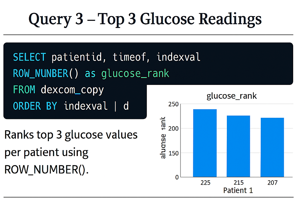
What the query does
Filters Dexcom rows to only EGV events (actual glucose values).
For each patient:
Sorts glucose values (indexval) from highest to lowest.
Assigns a rank using ROW_NUMBER().
Returns the top 3 highest glucose readings per patient.
This pattern is used for Identifying peak hyperglycemia events.
Comparing top glucose spikes across patients.
Question 4: Meal Nutrient Boundaries
Query: SELECT logged_food, GREATEST(calories::numeric, total_carbs::numeric) AS max_nutrient, LEAST(calories::numeric, total_carbs::numeric) AS min_nutrientFROM food_log;
T
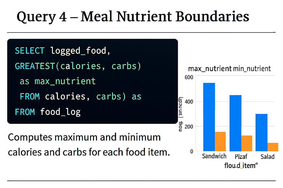
What it does:
This query compares calories and total carbs for each food by using GREATEST and LEAST to identify the dominant and secondary nutrient. It’s useful for nutrient‑balance analysis and quality checks. Optimization mainly involves ensuring numeric datatypes, removing unnecessary casts, and indexing if these computed values are used in filtering.
Question 5: Materialized View (Monthly HR Trends)
Query :
CREATE MATERIALIZED VIEW mv_monthly_hr_trends AS
SELECT
patientid,
DATE_TRUNC('month', timeof) AS month,
AVG(hr) AS avg_hr,
MIN(hr) AS min_hr,
MAX(hr) AS max_hr,
COUNT(*) AS reading_count
FROM hr_copy
GROUP BY patientid, DATE_TRUNC('month', timeof)
ORDER BY patientid, month;
Select * from mv_monthly_hr_trends;
REFRESH MATERIALIZED VIEW mv_monthly_hr_trends;
Output:
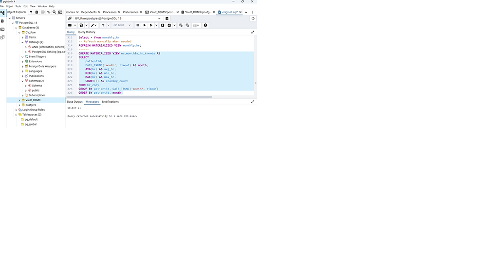

REASONING - Heart rate (HR) is a key physiological indicator in glycemic and metabolic health. Tracking HR trends month-to-month can reveal, changes in cardiovascular response to glucose variability, Effects of lifestyle or medication changes and Early signs of stress or complications in GVM patients.
OPTIMIZATION - Using a Materialized View for Monthly HR Trends allows you to precompute monthly averages, min/max, and counts for each patient.
Question6 : 23 Calculate Time Differences Measure intervals between consecutive readings
Query:
SELECT timeof, eda, timeof - LAG(timeof) OVER (PARTITION BY patientid ORDER BY timeof) AS time_diffFROM eda_table;

Breakdown of query
LAG() returns the timestamp of the previous EDA reading for that patient.
query computes per‑patient time gaps between consecutive EDA readings, and it becomes highly efficient with a (patientid, timeof) index plus optional clustering and filtering.
Thank you for taking time to read my blog.
Happy Querying!


