Breaking Down Decision Trees: A Simple Guide to Predicting the Future
- Pranjali Srivastava
- Aug 30
- 4 min read

Decision trees are versatile supervised learning algorithms used for both classification and regression tasks. They belong to the family of information-based learning methods, which rely on measures of information gain to guide their learning process. Decision trees can handle both continuous and categorical input and target features, making them suitable for a wide range of problems.
The core idea of decision trees is to identify the features that provide the most “information” about the target variable. By splitting the dataset based on these features, the algorithm aims to create subsets where the target variable is as pure as possible. The feature that results in the highest purity of the target variable is considered the most informative. This process of selecting the most informative feature and splitting the data continues iteratively until a predefined stopping criterion is met, at which point the process concludes at the leaf nodes.
The leaf nodes are where the decision tree makes predictions for new data. This works because the tree has learned patterns from the training data and can use those patterns to guess the target value (or class) for new, unseen data. A decision tree is made up of a root node (where the decision-making starts), interior nodes (where decisions are made based on features), and leaf nodes (which hold the final predictions). These nodes are connected by branches, showing the path from the root to the leaves.

The diagram might look simple and straightforward, but here is the challenge: how do you decide which feature or variable should become the root node and what comes next as the interior nodes?
In real-world scenarios, datasets often contain numerous variables, and figuring out the best way to split the data is the key to building an effective decision tree. The true power of a decision tree lies in the technique it uses to determine these splits. Only by using the right approach can you train the algorithm to make predictions with maximum accuracy.
These below examples will help you zoom out and understand the intricacies of the real time data –
House Price Prediction: It is based on features like location, number of bedrooms and square footage
Stock Market Analysis: Based on market factors like company revenue, global news sentiment and interest rate
Weather forecasting: Based on factors like humidity, wind speed and cloud cover
E-commerce revenue prediction: Based on features like website visit duration, number of items viewed, cart add and removal rate
Attribute Selection Measure (ASM) comes in the play to solve the issue of selecting the best attribute for root node and sub-nodes. It utilizes two of its types — Information gain and Entropy.
When building a regression decision tree for predicting house prices, we use ASM to decide the best splits in the data. Let’s break this down step by step with an example and illustrations.
Step 1: The Problem — Predicting House Prices
Imagine you have a dataset of houses with features like:
Location (City A, City B, City C)
Number of Bedrooms
Square Footage
The target variable is the price of the house. Your goal is to predict house prices based on these features.
Step 2: Understanding Entropy
Entropy, in a regression context, refers to the variance of the target variable (house prices) in a dataset. It can be considered as degree of randomness in the data. High entropy means the prices are spread out and unpredictable. Low entropy means the prices are tightly clustered and more predictable.
Example: Initial Entropy
Consider this small dataset:

Variance in Prices (Entropy):
The prices range from $300,000 to $450,000, so there’s a lot of spread. This is high entropy.
Step 3: Splitting to Reduce Entropy
To make better predictions, we split the dataset based on a feature that reduces entropy the most. This is where information gain comes in.
Information Gain Formula:
IG = Variance before split − Weighted Variance after split
Example: Splitting by Location
If we split the data by the “Location” feature:
City A:
Prices: $300,000, $350,000
Variance: Low (prices are close together)
City B:
Prices: $400,000, $450,000
Variance: Low
Weighted Variance After Split: Combine the variances of City A and City B, weighted by the number of houses in each city.
Information Gain: The difference between the initial variance (high) and the weighted variance after the split (low) tells us how much information we gained by splitting on “Location.”
Step 4: Iterative Splitting
After splitting by location, you can further reduce entropy by splitting within each group. For example:
In City A, split based on the number of bedrooms.
In City B, split based on square footage.
Each split reduces variance, making predictions more accurate.
Entropy measures the unpredictability (variance) in house prices, and information gain helps us decide the feature that reduces this unpredictability the most. By iteratively splitting the data, we build a tree that predicts house prices with high accuracy.
This method ensures the model focuses on the most important features step by step, improving the precision of its predictions.

Decision Tree Regression — Implementation in Python
Problem Statement: Use Machine Learning to predict the selling prices of houses based on few market factors. Build a model using Decision Tree in python
Importing required libraries and packages. Load the dataset and visualize using scatter plot to observe the entropy of feature.
Here, we are plotting house price against the area size of the house
import pandas as pd
import numpy as np
import matplotlib.pyplot as plt
from sklearn.tree import DecisionTreeRegressor
from sklearn.model_selection import train_test_split

data = pd.read_csv("Bengaluru_House_Data.csv")
plt.scatter(x=data['total_sqft'],y=data['price'],color='blue')
plt.xlabel('Area in squarefeet')
plt.ylabel('House price')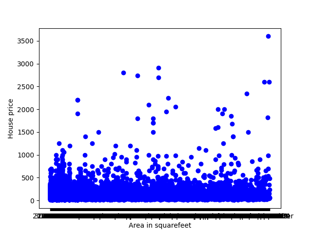
Define the features and target. Split the dataset into Train and Test sets
X = pd.DataFrame(data['total_sqft'])
Y = pd.DataFrame(data['price'])
x_trn, x_tst, y_trn, y_tst = train_test_split(X, Y, test_size = 0.20)
Build the model with the Decision Tree Regressor Function. The ‘criterion’ parameter of DecisionTreeRegressor has options — ‘absolute_error’, ‘poisson’, ‘squared_error’, ‘friedman_mse’
regressor = DecisionTreeRegressor(criterion='friedman_mse', random_state=100, max_depth=4, min_samples_leaf=1)
regressor.fit(x_trn,y_trn)
Predict the Values
y_pred = regressor.predict(np.array([1150]).reshape(1, 1))
print(y_pred)
Thus, for a house of area of 1150 sq. ft., the price predicted by model is Rs. 77.83 Lakh
Although, decision trees have some weakness like they are expensive to train and also there is a high chance of overfitting so as to perfectly fit all the samples. Random Forest Regression comes in play to resolve these issues as it combines the numerous decision trees into one model and average out the predictions of all individual decision tree.


