A Data Analyst's Guide to Cleaning Messy Data using PostgreSQL

We all know "messy data delivers messy insights". This isn't just a catchy phrase, it's the absolute truth. The quality of our final analysis is totally dependent on the quality of our source data. That's why preprocessing, or data cleaning, is the most critical first step of any project. It’s the work of transforming that raw, chaotic file into a reliable, clean resource we can actually trust.

So, to show you exactly what this cleaning process looks like, I've taken the Student Performance Dataset from Kaggle (Link to the dataset is given at the end of the blog post). It's a perfect example for us to work on. It's a powerful dataset, designed to help educators replace guesswork with data-driven action. But just like most raw data, it's messy. In this blog, I want to walk you through exactly how I tackled that critical first step. We'll be using PostgreSQL and pgAdmin to clean and prepare this dataset, turning it from a raw file into a reliable foundation for all the cool analysis that comes later.

Database Setup and Initial Load:

1: Setting Up Digital "Workbench":

Before we can clean any data, we need a place to put it. As I mentioned  I'll be using pgAdmin, which is the go-to graphical interface for PostgreSQL.

First, let's create a new, dedicated database for this project.

1. Once you have pgAdmin open, find the Databases tree in the left-hand browser.

2. Right-click on Databases and navigate to Create → Database.

3. A dialog box will pop up. I'm calling my database student_performance_predictions. I'm just leaving the Owner as the default, which is postgres.

Click Save, and our new database will appear in the browser tree.

2: Building the Table Structure:

Now that we have our database, we need to create a table inside it to hold our data.

To do this, we need to open the SQL editor:

1. Find the new student_performance_predictions in the browser.

2. Right-click on it and select the Query Tool.

This opens a blank editor panel, which is where we'll tell PostgreSQL how to build our table. We are going to paste in the CREATE TABLE script I prepared. This script defines all the column names and, importantly, what type of data each column is supposed to hold.

Here's the query I used to build the student_raw table:

3: Getting Our Data into the Table:

Okay, so we've successfully executed our query, and now we have a perfectly structured, but completely empty, student_raw table. Now we need to load our actual data (from a .csv file) into it. The simplest method is to just use the built-in pgAdmin import tool.

1. Find the student_raw table in the browser tree on the left.

2. Right-click on the table name.

3. In the menu, find and select Import/Export.

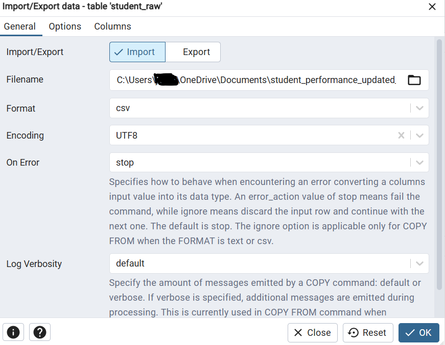
4. A new window will pop up. Here's what to do:

   • Toggle Import at the top.

   • Filename: Click the button to browse your computer and select your .csv file.

   • Format: Make sure this is set to csv.

   • Header: This is important! Toggle this to Yes so that pgAdmin knows the first row of your file contains column names and not data.

5. Click OK.

   
   

   Once it's finished, you should see a success notification.

4: Inspecting the "Raw" Data

Now that the data is loaded, let's run a quick check to see what we're really working with.

SELECT * FROM student_raw LIMIT 20;

This gives a quick overview of the kind of data in each column.

Just from this quick peek, we can already see some... issues. Our next step is to confirm the table's structure with information_schema. This is like looking at the blueprint of the table.

SELECT

    column_name,

    data_type,

    is_nullable,

    column_default

FROM

    information_schema.columns

WHERE

    table_name = 'student_raw';

When we run the information_schema query, it confirms the blueprint we just created. You'll see every data_type is character varying (text). Now, here I deliberately set it up this way in our CREATE TABLE script, because this is the most common, real-world problem we will face. Often, when importing a messy CSV, the safest (or only) way to get the data loaded without errors is to treat every column as text first. Many import tools even do this by default. So, the student_raw table perfectly represents this "raw" state. This is the core problem we're here to solve. We can't do any math or proper analysis on these text fields. Now we can go ahead and clean our data.

Data Cleaning Workflow:

Step 1: The Golden Rule - Never Edit Your Raw Data:

Our first step is always to copy the raw data. That way, the original file is always safe and untouched. The first thing is to create a copy of the table. All the cleaning work will happen on this new student_cleaned table.

Step 2: Remove Identical Row Duplicates

First real cleaning step is to remove any 100% identical duplicates. We should do this at the very beginning—I can't recommend it enough. It's just more efficient. There's no point in cleaning data that you're just going to delete later. To do this, we use a handy PostgreSQL feature called ctid. Think of it as a secret, unique ID for every single row. The method is simple: We tell PostgreSQL to group all the rows that are perfect matches. Then, for each group, it finds the 'first' one (using MIN(ctid)) and deletes all the others. This one query gets rid of all the exact copies, letting me focus on the data that matters.

This message is great news! It means the data was already unique at the row level, which is one less problem for me to worry about.

Step 3:  Converting Text Nulls to Real Nulls

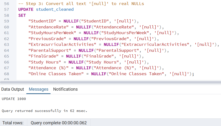
When we look back at the table structure (Inspecting data) and look at the data, we can see missing values weren't NULL (the database way of saying "empty"). Instead, they were the text string '[null]'.

This is a critical problem. If we try to convert the 'PreviousGrade' column to a number, the database will hit '[null]' and fail. Before we can fix the data types, we must convert these text strings into real NULL values. The NULLIF function is perfect for this. It literally means: "If you see the value '[null]', replace it with NULL. Otherwise, leave it alone."

Step 4: Fix All Data Types

This is the most important step for making data usable. As we saw every column was imported as VARCHAR (text). We can't average a text column!

Now that we have gotten rid of the '[null]' text, we can safely convert these columns. We will use ALTER TABLE with the USING clause. This USING part is where the magic happens—it tells PostgreSQL how to make the conversion.

• ::INTEGER converts the text to a whole number.

• ::NUMERIC converts it to a number with decimals.

• ::BOOLEAN is smart and understands that 'True', 'yes', and '1' all mean TRUE.

  
  

  

  

Now, our data structure is finally correct.

Step 5: Handle StudentID Duplicates & Set the Primary Key

Okay, we've handled identical rows, but now we have to deal with logical duplicates. What if we have two rows with the same "StudentID" but different grades?

First, any row without a "StudentID" is not useful for tracking student performance, so we will just delete those.

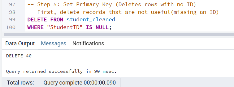
This message tells us that the query found and successfully deleted 40 rows that had a NULL value in the "StudentID" column. That's 40 rows of data that are not useful are gone, which makes our dataset much cleaner.

Now that we've cleared out the "noise," we're left with only the rows that have a StudentID. This means we can finally focus on the real challenge: finding and removing the duplicate StudentIDs.

Now we have to make a choice. What do we do with two rows that have the same StudentID? In a real-world project, we might check with the data owner. But for this, we need to set a simple rule. The rule will be: the first row wins. We'll keep the very first record the database has for each student and delete any other copies that share that ID. The ctid trick is perfect for this. We will use the exact same query as before, but this time we will only GROUP BY "StudentID". This tells PostgreSQL to find the 'first' row for each student and delete all the rest."

This message tells us that my query found and deleted 44 rows that were logical duplicates. These were rows that had a valid StudentID, but that ID already existed in another row. By making the tough call to keep only one version of each student, we've just solved our data integrity problem. Now, after both of our delete operations, we can be 100% confident that every single row in my student_cleaned table has a StudentID and that every single StudentID appears only once.

Our dataset is finally ready for its Primary Key.

Our data integrity is now locked in. This command will also fail if any duplicates remain, so it's a great final check.

Step 6: Impute Missing Values.

Our data structure is solid, but we still have those real NULLs we created in Step 3. For analysis, it's often better to fill these gaps with a logical default. This is called "imputing." We will use COALESCE, which is one of my favorite functions. It just returns the first non-null value it finds. So, COALESCE("PreviousGrade", 0) means "Give me the PreviousGrade. If it's NULL, give me 0 instead."

(Note: We are not cleaning “Study Hours” or “Attendance (%)” because, as we will see in a bit, they’re redundant and we will drop them.)

Step 7: Standardize Categorical Data

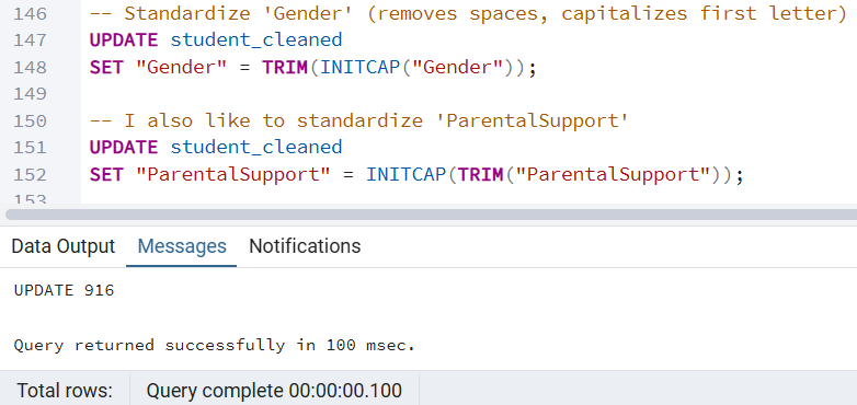
This is the final polish. The Gender column might have 'Male', 'male', and ' Male '. Our analysis will treat those as three different categories! We will use TRIM to remove whitespace and INITCAP to make the first letter capital and the rest lowercase. This ensures ' male ' and 'MALE' both become 'Male'.

Step 8: Fix Illogical Values.

he data types are right, but are the values logical? For example: A student can't have 110% attendance or study for -5 hours. Lets address this.

When I ran this, I got UPDATE 0. No records were updated, which is great news! It means the data didn't have these specific illogical values, but it's always a step worth taking.

Step 9: Final Cleanup (Drop Redundant Columns and Column Renaming)

Last step! First, while cleaning, we can notice that the table has duplicate columns. "Study Hours" looks just like "StudyHoursPerWeek", and "Attendance (%)" is a copy of "AttendanceRate". These will just cause confusion, so we will drop them.

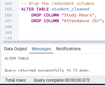
With those gone, our table only has the columns we need. But this brings us to the second part of the final polish: the column names. If we look at the table, you'll see names like FinalGrade, StudentID, and ParentalSupport. This is going to be a pain. Because they have capital letters (or spaces, which we've also seen), we will be forced to use double-quotes (") every single time we write a query.

For example, we would have to write: SELECT "FinalGrade", "StudyHoursPerWeek" ...

If we forget the quotes and just type SELECT finalgrade..., our query will fail. This is a constant, tiny annoyance that we rather just fix forever. This is why the "gold standard" for SQL databases is to use snake_case. It means everything is lowercase, with underscores instead of spaces (e.g., final_grade). So, we will run one last ALTER TABLE command to rename all the remaining columns. This is the ultimate final polish. It makes the table not just clean, but an absolute pleasure to use.

And... We're Done!

All our queries from here on out will be simple, clean, and fast to type, with no double-quotes required. Now the dataset is clean. We've taken that messy, unreliable student_raw table and transformed it into the trustworthy, structured, and efficient student_cleaned table.

Let's take one final look:

SELECT * FROM student_cleaned LIMIT 20;

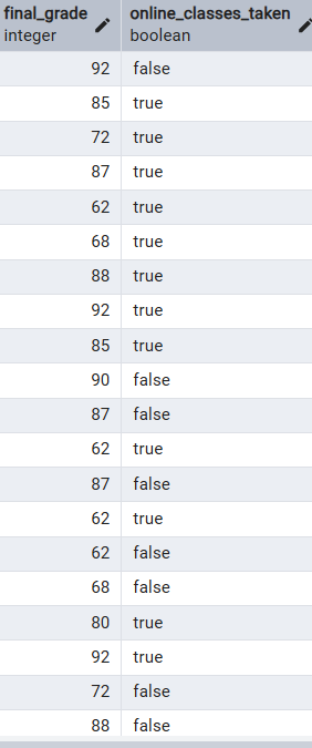
It's beautiful. We have successfully transformed a raw, messy, and unreliable dataset into a trustworthy, structured, and efficient table.

Let's do a final check. Look at what we've accomplished:

• Clean & Consistent Names: All columns are now in simple snake_case (like final_grade and student_id). We will never have to use double-quotes for these columns again.

• Correct Data Types: The headers tell the story. final_grade is a proper integer, study_hours_per_week is numeric, and online_classes_taken is a clean boolean. We can finally run calculations on this data.

• Primary Key: The student_id column is our primary key. We know the data is 100% unique for each student, and the database will enforce that rule.

• Clean, Standardized Text: The parental_support column is clean and consistent. There are no weird capitalizations or spaces.

• No Missing Values: Every row is complete, filled with our logical defaults.

  
  

Now we are finally ready to do the fun part which is the analysis! Happy Querying!!

**Dataset: https://www.kaggle.com/datasets/haseebindata/student-performance-predictions?resource=download